Autoencoders

An autoencoder is a type of a neural network used to learn, in an unsupervised way, a compressed data representation by matching its input to its output. An efficient compression is archived by minimizing the reconstruction error.

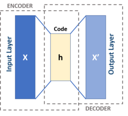Michela Massi, CC BY-SA 4.0, via Wikimedia Commons

An autoencoder consists of two parts, the encoder $\phi:\mathcal{X} \rightarrow \mathcal{Z}$ and the decoder $\theta: \mathcal{Z} \rightarrow \mathcal{X}$, which can be defined as transitions

$$\phi,\theta = \underset{\phi,\theta}{\operatorname{arg,min}}, |\mathcal{X}-(\theta \circ \phi) \mathcal{X}|^2$$

where the encoder stage of an autoencoder takes the input $\mathbf{x} \in \mathbb{R} ^{d}={\mathcal {X}}$ and maps it to $\mathbf{h} \in \mathbb {R}^{p}={\mathcal{Z}}$.

Experiment Setup

Here, we define the common parameters of our autoencoder. A dimensions of network hidden layers and compressed represintation, as well as the learing rate for the optimization.

using Flux
device = cpu # where will the calculations be performed?
L1, L2 = 128, 8 # layer dimensions
η = 0.01 # learning rate for ADAM optimization algorithm
batch_size = 100; # batch size for optimization

We’ll use MNIST dataset for our experiments with autoencoders. This dataset consists of 60000 $28 \times 28$ pixel images of handwritten digits.

using Flux.Data, MLDatasets
function get_data(batch_size)
    xtrain, _ = MLDatasets.MNIST.traindata(Float32)
    d = prod(size(xtrain)[1:2]) # input dimension
    xtrain1d = reshape(xtrain, d, :) # reshape input as a 784-dimesnonal vector (28*28)
    dl = DataLoader(xtrain1d, batchsize=batch_size, shuffle=true)
    dl, d
end

dl, d = get_data(batch_size)

(DataLoader{Matrix{Float32}, Random._GLOBAL_RNG}(Float32[0.0 0.0 … 0.0 0.0; 0.0 0.0 … 0.0 0.0; … ; 0.0 0.0 … 0.0 0.0; 0.0 0.0 … 0.0 0.0], 100, 60000, true, 60000, [1, 2, 3, 4, 5, 6, 7, 8, 9, 10  …  59991, 59992, 59993, 59994, 59995, 59996, 59997, 59998, 59999, 60000], true, Random._GLOBAL_RNG()), 784)

We add an auxiliary function for displaying images produced by our autoencoders.

using Images
img(x::AbstractVector) = Gray.(reshape(clamp.(x |> cpu, 0, 1), 28, 28))

img (generic function with 1 method)

Take a sample of the dataset and display it.

data_sample = dl |> first |> device;
img_sample = [i for i in eachcol(data_sample[:,1:7])]
img.(img_sample)

Define simple training function for our experiments which relies on Flux.jl automatic differentiation and (stochastic) gradient optimization framework.

function train!(model_loss, model_params, opt, loader, epochs = 10)
    train_steps = 0
    "Start training for total $(epochs) epochs" |> println
    for epoch = 1:epochs
        print("Epoch $(epoch): ")
        ℒ = 0
        for x in loader
            loss, back = Flux.pullback(model_params) do
                model_loss(x |> device)
            end
            grad = back(1f0)
            Flux.Optimise.update!(opt, model_params, grad)
            train_steps += 1
            ℒ += loss
        end
        println("ℒ = $ℒ")
    end
    "Total train steps: $train_steps" |> println
end

train! (generic function with 2 methods)

Dense Autoencoder

We begin with a deep dense autoencoder in which an encoder $\phi$ and a decoder $\phi$ represented by neural networks: 2 layers for an encoder and 2 layers for a decoder. In total, we got a deep neural network that is composed of the 4 layers which perform following transformation: $$\mathbb{R}^{784} \to \mathbb{R}^{128} \to \mathbb{R}^{8} \to \mathbb{R}^{128} \to \mathbb{R}^{784}$$

So the original 784-dimensional data compressed to the 8-dimensional representation.

enc1 = Dense(d, L1, leakyrelu)
enc2 = Dense(L1, L2, leakyrelu)
dec3 = Dense(L2, L1, leakyrelu)
dec4 = Dense(L1, d)
m = Chain(enc1, enc2, dec3, dec4) |> device

Chain(Dense(784, 128, leakyrelu), Dense(128, 8, leakyrelu), Dense(8, 128, leakyrelu), Dense(128, 784))

Define the reconstruction loss function as mean square error, $|(\theta \circ \phi) x - x |^2$.

loss(x) = Flux.Losses.mse(m(x), x)
loss(data_sample)

0.11730117f0

Setup optimizer parameters and train network for 5 epochs.

opt = ADAM(η)
ps = Flux.params(m) # parameters
train!(loss, ps, opt, dl, 5)

Start training for total 5 epochs
Epoch 1: ℒ = 26.156715
Epoch 2: ℒ = 19.408918
Epoch 3: ℒ = 18.337896
Epoch 4: ℒ = 17.72952
Epoch 5: ℒ = 17.113337
Total train steps: 3000

Generate a sample from the output of the autoencoder.

img.(map(m, img_sample))

Variational Autoencoder

Variational autoencoders (VAE) are variational Bayesian methods with a multivariate distribution as prior, and a posterior approximated by an artificial neural network.

Given a dataset $\mathcal{X}$ and a multivariate latent encoding space $\mathcal{Z}$, the objective is to model the data as a distribution $p_\theta(\mathbf{x})$ with $\theta$ defined as the set of the network parameters, such that

\begin{equation}\label{eq:latent-model} p_\theta(\mathbf{x}) = \int_\mathcal{Z} p_\theta(\mathbf{x|z}) p(\mathbf{z}) d\mathbf{z} \end{equation}

where $\mathbf{x} \in \mathcal{X}$ and $\mathbf{z} \in \mathcal{Z}$. The calculations of $p_\theta(\mathbf{x})$ as well as the true posterior for the latent variables $p_\theta(\mathbf{z|x}) = p_\theta(\mathbf{x|z})p(\mathbf{z})/p_\theta(\mathbf{x})$ are intractable. Thus, it’s necessary to approximate the posterior by introducing probabilistic encoder $q_\phi(\mathbf{z|x}) \approx p_\theta(\mathbf{z|x})$.

The encoder portion of a VAE yields an approximated posterior distribution $q_\phi(\mathbf{z|x})$, and is parametrized on a neural network by weights collectively denoted $\phi$, and similarly, the decoder portion of VAE produces a likelihood distribution $p_\theta(\mathbf{x|z})$, and is parametrized on a neural network by weights $\theta$.

The Variational Bound

The parameters of the neural networks are estimated to maximize the marginal likelihood of the input data, $p_\theta(\mathbf{x})$. The likelihood maximized under a variational Bayesian approximation, making the optimization problem amenable to the backpropagation algorithm required for updating the network parameters, as follows:

\begin{equation}\label{eq:var-approx} \log p_\theta(\mathbf{x}) = \mathbb{KL} [ q_\phi(\mathbf{z|x}) || p_\theta(\mathbf{z|x}) ] + \mathbb{E}{\mathbf{z} \sim q\phi(\mathbf{z|x})}[p_\theta(\mathbf{x|z})] - \mathbb{KL} [ q_\phi(\mathbf{z|x}) || p(\mathbf{z}) ] \end{equation} where $\mathbb{KL}$ is the Kullback–Leibler divergence.

In the right-hand side of $\eqref{eq:var-approx}$, the first term measures the distance between the approximate and the true unknown posterior, the second term is the reconstruction error, and the third term is the KL divergence between the encoder distribution and a known prior. The last two terms of $\eqref{eq:var-approx}$ represent the variational lower bound. Maximizing the bound will be approximately equivalent to maximizing the marginal likelihood [1].

Reparametrization

The second term of $\eqref{eq:var-approx}$, the stochastic sampling, through which it is possible to sample from the latent space and feed the probabilistic decoder, is the non-differentiable operation. It requires reparameterization to work with the backpropagation algorithm. Let the variational approximate posterior be a multivariate Gaussian with a diagonal covariance structure:

$$\log q_\phi( \mathbf{z}|\mathbf{x}{(i)} ) = \log \mathcal{N}(\mathbf{z}| \mathbf{\mu}{(i)}, \mathbf{\sigma}^2_{(i)} \mathbf{I})$$ where the mean and the diagonal variance of the approximate posterior are outputs of the non-linear encoding of data point $\mathbf{x}_{(i)}$ and the variational parameters $\phi$.

Thus, we sample from the posterior $\mathbf{z_{}}{(i)} \sim q\phi( \mathbf{z}|\mathbf{x}{(i)} )$ using $\mathbf{z{}}{(i)} = \phi(\mathbf{x}{(i)},\epsilon) = \mathbf{\mu}{(i)} + \sigma{(i)} \odot \epsilon$ where $\epsilon \sim \mathcal{N}(0, \mathbf{I})$ and $\odot$ denotes the Hadamard product [1].

Construct variational autoencoder network with Guassian encoder.

encoder = Chain(Dense(d, L1, leakyrelu), Parallel(tuple, Dense(L1, L2), Dense(L1, L2))) |> device
decoder = Chain(Dense(L2, L1, leakyrelu), Dense(L1, d)) |> device
encoder, decoder

(Chain(Dense(784, 128, leakyrelu), Parallel(tuple, Dense(128, 8), Dense(128, 8))), Chain(Dense(8, 128, leakyrelu), Dense(128, 784)))

Perform reconstruction of the input, and return model parameters as well

function reconstuct(x)
    μ, logσ = encoder(x) # decode posterior parameters
    ϵ = device(randn(Float32, size(logσ))) # sample from N(0,I)
    z = μ + ϵ .* exp.(logσ) # reparametrization
    μ, logσ, decoder(z)
end

reconstuct (generic function with 1 method)

Define loss function of variational autoencoder with regularization

Flux.Zygote.@nograd Flux.params
function vae_loss(λ, x)
    len = size(x)[end]
    μ, logσ, decoder_z = reconstuct(x)

    # D_KL(q(z|x) || p(z|x))
    kl_q_p = 0.5f0 * sum(@. (exp(2f0 * logσ) + μ^2 - 1f0 - 2f0 * logσ)) / len # from (10) in [1]

    # E[log p(x|z)]
    logp_x_z =  -Flux.Losses.logitbinarycrossentropy(decoder_z, x, agg=sum)/len

    # regularization
    reg = λ * sum(x->sum(x.^2), Flux.params(decoder))

    -logp_x_z + kl_q_p + reg
end

vae_loss (generic function with 1 method)

λ = 0.005f0
loss(x) = vae_loss(λ, x)
loss(data_sample)

549.64185f0

Setup optimizer parameters and train network for 5 epochs.

opt = ADAM(η) # optimizer
ps = Flux.params(encoder, decoder) # parameters
train!(loss, ps, opt, dl, 5)

Start training for total 5 epochs
Epoch 1: ℒ = 95935.95
Epoch 2: ℒ = 82061.76
Epoch 3: ℒ = 80723.4
Epoch 4: ℒ = 79984.555
Epoch 5: ℒ = 79640.5
Total train steps: 3000

Display a sample from the dataset.

reconst = [reconstuct(i) for i in img_sample]
img.(map(last, reconst))

Wasserstein Autoencoder

One problem with VAE that there is no guarantee that the learned latent space is distributed according to the assumed prior distribution, such that, the aggregated posterior distribution $q_\phi (\mathbf{z}) = \mathbf{E}{\mathbf{x} \sim \mathcal{X}} q\phi(\mathbf{z|x})$ doesn’t to conform well to $p(\mathbf{z})$ after training which results in a blurry output [2].

Wasserstein autoencoder (WAE) tries to fix the above problem by minimizing optimal transport between the data distribution $P_X$ with the density $p(\mathbf{x})$ and the latent prior model $P_Z$ with the density $p(\mathbf{z})$, s.t.

$$ W_{c}(P_X, P_Z) = \inf_{\Gamma \in \Pi(x \sim P_X,z \sim P_Z)} \mathbb{E}_{(\mathbf{x},\mathbf{z}) \sim \Gamma}[c(\mathbf{x},\mathbf{z})] $$

where $c:\mathcal{X} \times \mathcal{X} \to \mathcal{R}_+$ is any measurable cost function.

For example, if $c(x, y) = d(x, y) = |x-y|$ then the above problem has a dual Kantorovich-Rubinstein formulation (or 1-Wasserstein distance):

\begin{equation}\label{eq:1wasserstein} W_1(P_X, P_Z) = \sup_{f \in \mathcal{F}L} \mathbb{E}{\mathbf{x} \sim P_X}[f(x)] - \mathbb{E}_{\mathbf{z} \sim P_Z}[f(z)] \end{equation}

where $\mathcal{F}_L$ is a class of all bounded 1-Lipschitz functions on a metric space $(\mathcal{X} , d)$.

The optimal cost between $P_X$ and $P_Z$ can be simplified to the transportation plan factors through the map $G:\mathcal{Z} \to \mathcal{X}$ under a conditional distribution $q(\mathbf{z|x})$ such that its marginal distribution $Q_Z$ with the density $q(\mathbf{z}) = \mathbf{E}_{\mathbf{x} \sim P_X} q(\mathbf{z|x})$ is identical to the prior $P_Z$ with the density $p(\mathbf{z})$, s.t.

$$ \inf_{\Gamma \in \Pi(x \sim P_X,z \sim P_Z)} \mathbb{E}{(\mathbf{x},\mathbf{z}) \sim \Gamma}[c(\mathbf{x},\mathbf{z})] = \inf{q(\mathbf{z}) = p(\mathbf{z})}\mathbb{E}{\mathbf{x} \sim P_X} \mathbb{E}{\mathbf{z} \sim q(\mathbf{z|x})}[c(\mathbf{x},G(\mathbf{z}))] $$

For a numerical solution, a relaxation of the constraints on $q(\mathbf{z})$ by adding a penalty to the objective leads to the WAE objective:

$$ \inf_{q(\mathbf{z|x}) \in \mathcal{Q}}\mathbb{E}{\mathbf{x} \sim P_X} \mathbb{E}{\mathbf{z} \sim q(\mathbf{z|x})}[c(\mathbf{x},G(\mathbf{z}))] + \lambda \mathcal{D}(Q_Z, P_Z)$$

where $\mathcal{Q}$ is any nonparametric set of probabilistic encoders, which provide the latent codes to the decoder informative enough to reconstruct the encoded training examples, $\mathcal{D}(Q_Z, P_Z)$ is an arbitrary divergence that matches the encoded distribution of training examples $Q_Z$ to the prior $P_Z$, and $\lambda > 0$ is a hyperparameter.

WAE formulation allows the encoder to be deterministic as well as Gaussian. We choose Gaussian encoder to make a comparison with VAE results.

encoder = Chain(Dense(d, L1, leakyrelu), Parallel(tuple, Dense(L1, L2), Dense(L1, L2))) |> device
decoder = Chain(Dense(L2, L1, leakyrelu), Dense(L1, d)) |> device
encoder, decoder

(Chain(Dense(784, 128, leakyrelu), Parallel(tuple, Dense(128, 8), Dense(128, 8))), Chain(Dense(8, 128, leakyrelu), Dense(128, 784)))

The fallowing function, similar to VAE, generates output the input data given the approximate prior parameters from Gaussian encoder.

function reconstuct(x)
    μ, logσ = encoder(x) # decode posterior parameters
    ϵ = device(randn(Float32, size(logσ))) # sample from N(0,I)
    z = μ + ϵ .* exp.(logσ) # reparametrization
    μ, logσ, z, decoder(z)
end

reconstuct (generic function with 1 method)

The penalty $\mathcal{D}(Q_Z, P_Z)$ is defined in form of the maximum mean discrepancy (MMD) statistic as follows

$$ MMD_k(P_Z, Q_Z) = \left | \int_\mathcal{Z} k(\mathbf{z}, \cdot) d p(\mathbf{z}) - \int_\mathcal{Z} k(\mathbf{z}, \cdot) d q(\mathbf{z}) \right |_{\mathcal{H}_k} $$

where $k : \mathcal{Z} \times \mathcal{Z} \to \mathcal{R}$ is a positive-definite reproducing kernel, and $\mathcal{H}_k$ is the RKHS of real-valued functions mapping $\mathcal{Z}$ to $\mathcal{R}$. MMD has an unbiased estimator, which can be used with stochastic gradient descent (SGD) methods. The MMD statistic is an unbiased estimator of the distance $\eqref{eq:1wasserstein}$.

We need some auxiliary functions for determining the WAE loss function.

using LinearAlgebra, Statistics
#using CUDA
#Flux.Zygote.@nograd CUDA.sort!
Flux.Zygote.@nograd sort!

normsq(x) = norm.(eachcol(x)).^2 |> device
function distance(x::AbstractMatrix)
    norm_x = normsq(x)
    norm_x .+ norm_x' - 2*x'*x
end
function distance(x::AbstractMatrix, y::AbstractMatrix)
    norm_x, norm_y = normsq(x), normsq(y)
    norm_x .+ norm_y' - 2*x'*y
end

distance (generic function with 2 methods)

Here is an implementation of the WAE loss function.

reconstruction_loss(x, y) = mean(normsq(x - y))

function mmd_penalty(pz, qz) # with RBF kernel
    n = size(pz,2)
    n² = n*n
    n²1 = n²-n
    hlf = n²1 >> 1
    dist_pz = distance(pz)
    dist_qz = distance(qz)
    dist = distance(pz,qz)

    σₖ² = sort!(dist[:])[hlf]
    σₖ² += sort!(dist_qz[:])[hlf]    

    sum(exp.(dist_qz ./ -2σₖ²) + exp.(dist_pz ./ -2σₖ²) - 2I)/n²1 -
        2*sum(exp.(dist ./ -2σₖ²))/n²
end

function wae_loss(λ, x)
    μ, logσ, smpl_qz, y = reconstuct(x)
    smpl_pz = device(randn(Float32, size(smpl_qz)...))
    reconstruction_loss(x, y) + λ*mmd_penalty(smpl_pz, smpl_qz)
end

λ = 10.0f0
loss(x) = wae_loss(λ, x)
loss(data_sample)

110.71296f0

Setup optimizer parameters and train network for 5 epochs.

opt = ADAM(η) # optimizer
ps = Flux.params(encoder, decoder) # parameters
train!(loss, ps, opt, dl, 5)

Start training for total 5 epochs
Epoch 1: ℒ = 15915.853
Epoch 2: ℒ = 12841.568
Epoch 3: ℒ = 12501.018
Epoch 4: ℒ = 12185.054
Epoch 5: ℒ = 12037.139
Total train steps: 3000

Now, we display a sample passed through the WAE reconstruction.

reconst = [reconstuct(i) for i in img_sample]
img.(map(last, reconst))

References

[1] Kingma, Diederik P., and Max Welling. *Auto-encoding variational bayes.* arXiv:1312.6114, 2013.[2] Tolstikhin, Ilya, Olivier Bousquet, Sylvain Gelly, and Bernhard Schoelkopf. *Wasserstein auto-encoders.* arXiv:1711.01558, 2017.