Introduction
Mixture models are used for many purposes in data science, e.g. to represent feature distributions or spatial relations. Given a fixed data sample, one can fit a mixture model to it using one of a variety of methods. A very common mixture structure is based on Gaussian distributions, the Gaussian Mixture Model (GMM). The expectation-minimization (EM) algorithm allows to find GMM parameters by maximizing model’s likelihood. This approach usually requires closed-form description of parameters’ estimates and have slow convergence to optimal solution. These limitation can be overcome by using (quasi-)Newton optimization. In conjunction with automatic differentiation (AD), finding optimal model parameters become trivial.
For modeling a collection of time series, another model based on a mixture of ARMA processes, Mixture of ARMA Models, can be used. Using similar MLE optimization and AD approach, we will show how to cluster time series.
Gaussian Mixture Model
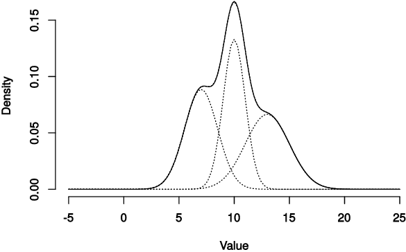
A Gaussian mixture is a distribution $p(\boldsymbol x | \boldsymbol \Phi)$ in $\mathbb{R}^d$ with a density composed of weighted sum of $k$ Gaussian densities of the following form:
\begin{equation} \label{eq:gmm} p(\boldsymbol x | \boldsymbol \Phi) = \sum_{i=1}^{k} \pi_i p(\boldsymbol x | \boldsymbol \mu_i, \boldsymbol \Sigma_i) \end{equation}
where $\boldsymbol \Phi = {\boldsymbol \mu_1, \ldots, \boldsymbol \mu_k, \boldsymbol \Sigma_1, \ldots, \boldsymbol \Sigma_k, \pi_1, \ldots, \pi_k}$, $\pi_k = 1 - \sum_{i=1}^{k-1}\pi_{i}$, and
\begin{equation} \label{eq:gaussian} p(\boldsymbol x | \boldsymbol \mu_i, \boldsymbol \Sigma_i) = \frac{1}{\sqrt{(2\pi)^d |\boldsymbol \Sigma_i|}} e^{-\frac{1}{2}(\boldsymbol x - \boldsymbol \mu_i)^T \boldsymbol \Sigma_i^{-1} (\boldsymbol x - \boldsymbol \mu_i)} \end{equation}
The log of the likelihood function for $\eqref{eq:gmm}$ is
\begin{equation} \label{eq:ll-gmm} \ln p(\boldsymbol x | \boldsymbol \Phi) = \ln \sum_{i=1}^{k} \pi_i p(\boldsymbol x | \boldsymbol \mu_i, \boldsymbol \Sigma_i) \end{equation}
Because of the sum operation under the logarithm, we cannot produce a closed form solution for maximization of $\eqref{eq:ll-gmm}$ for $\boldsymbol \Phi$. The common way to find MLE of $\boldsymbol \Phi$ is the Expectetion-Maximization (EM) algorithm [1].
Instead of EM, we use Newton’s optimization with automatic differentiation feature to find MLE of our GMM. Since Newton’s method converges only locally, one needs to provide good starting values. For this purpose we use a gradient descent algorithm for a few iterations.
Reparametrization
We need to ensure that parameters of the likelihood function $\boldsymbol \Phi$ convergence to the valid values during optimization, so we reparametrize them to avoid inequality constraints as follows [3].
In order for prior probability $\pi_i$ values stay in the interval $[0;1]$, we rewrite them as follows: \begin{equation} \label{eq:prior-reparam} \pi_i = \pi_i(\boldsymbol q) = \frac{q_i^2}{q_1^2+\cdots+q_{k-1}^2+1} \end{equation} where $\boldsymbol q = (q_1, \ldots, q_{k-1})$ and $\pi_k(q) = 1 - \sum_{i=1}^{k-1} \pi(q_i)$.
The covariance matrix for Gaussian distribution and its inverse need to be symmetric positive-definite. Using this properties we can use Cholesky decomposition to rewrite the covariance term as $$\Sigma_i^{-1} = L_i L_i^T$$ where the diagonal elements of $L_i$ are not zeros.
Thus multivariate normal probability density function parametrized by $\mu$ and $L$ is \begin{equation}\label{eq:gaussian-reparam} p(\boldsymbol x | \boldsymbol \mu_i, \boldsymbol L_i) = \frac{1}{\sqrt{(2\pi)^d }}|\boldsymbol L_i| e^{-\frac{1}{2}(\boldsymbol x - \boldsymbol \mu_i)^T \boldsymbol L_i L_i^T (\boldsymbol x - \boldsymbol \mu_i)} \end{equation}
And the GMM log-likelihood becomes \begin{equation} \label{eq:ll-gmm-reparm} \ln p(\boldsymbol x | \boldsymbol \Phi) = \ln \sum_{i=1}^{k} \pi_i(\boldsymbol q) p(\boldsymbol x | \boldsymbol \mu_i, \boldsymbol L_i) \end{equation} where $\boldsymbol \Phi = {\boldsymbol \mu_1, \ldots, \boldsymbol \mu_k, \boldsymbol L_1, \ldots, \boldsymbol L_k, q_1, \ldots, q_{k-1}}$.
include("misc.jl") # add some auxiliary functions
Let’s define a prior function that implements $\pi_i(\boldsymbol q)$:
function prior(q::AbstractVector)
    ret = q.^2 ./ (sum(abs2, q) + 1)
    [ret..., 1 - sum(ret)]
end

let qs = abs.(randn(3))*10
    @show qs
    @show prior(qs)
    @show sum(prior(qs))
end;
qs = [9.883767254426916, 5.124153615374239, 18.33616531975445]
prior(qs) = [0.2118325381422205, 0.05693665272719697, 0.7290623679318468, 0.0021684411987357155]
sum(prior(qs)) = 1.0
The Gaussian log probability density function implementation is following:
function lognormal(x::AbstractVector, μ, L)
    d = length(x)
    C = -d*log2π/2
    z = x .- μ
    Σ⁻¹ = L*L'
    dis = z'*Σ⁻¹*z
    C + logdet(L) - dis/2
end

let x = ones(2),
    μ = zeros(2),
    Σ = Symmetric([1.0 0.2; 0.2 1.0]),
    L = cholesky(inv(Σ)).L

    @show logpdf(MvNormal(μ, Σ), x)
    @show lognormal(x, μ, L)
end;
logpdf(MvNormal(μ, Σ), x) = -2.6507994024825514
lognormal(x, μ, L) = -2.6507994024825514
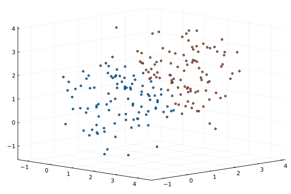
Example
Our example model has two mixture components with prior probability 0.5. The mixture Gaussians distributions have following parameters:
- $\mu_1 = (1 ; 1 ; 1)^T$, $\mu_2 = (2 ; 2 ; 2)^T$
- $\Sigma_1 = \Sigma_2 = \left[\begin{matrix} 1 & 0.2 & 0.2 \ 0.2 & 1 & 0.2 \ 0.2 & 0.2 & 1 \end{matrix}\right]$
Let’s define our model and generate some sample data.
k, d, n = 2, 3, 200
μ1, μ2 = ones(d), 2ones(d)
Σ1, Σ2 = [Symmetric([1.0 0.2 0.2; 0.2 1.0 0.2; 0.2 0.2 1.0]) for i in 1:2]
p1, p2 = 0.5, 0.5
M = build_model([μ1, μ2],[Σ1, Σ2],[p1, p2])
MixtureModel{FullNormal}(K = 2)
components[1] (prior = 0.5000): FullNormal(
dim: 3
μ: [1.0, 1.0, 1.0]
Σ: [1.0 0.2 0.2; 0.2 1.0 0.2; 0.2 0.2 1.0]
)

components[2] (prior = 0.5000): FullNormal(
dim: 3
μ: [2.0, 2.0, 2.0]
Σ: [1.0 0.2 0.2; 0.2 1.0 0.2; 0.2 0.2 1.0]
)
Random.seed!(1)
xs = rand(M, n)
3×200 Matrix{Float64}:
 0.532758  2.16588  0.0190413  1.66579  …  1.06266  1.48708  2.38837
 1.39592   2.16497  0.424957   1.46917     1.65382  1.33157  2.20693
 1.2431    1.47679  0.626154   2.11146     2.01407  2.74777  1.30784
A “hard” probabilistic classifier allows to partition our dataset, and indicate from which component of the mixture a point is originated.
using Plots
default(fmt = :png)
scatter(xs[1,:],xs[2,:],xs[3,:], markersize=2.0, cam=(45,30), c=predict(M,xs), ms=3, leg=:none)
For MLE optimization, we want to define an optimization function, the log-likelihood over our dataset. For the log-likelihood function parameters are represented as a single vector, to comply with ForwardDiff.jl limitations on the argument form. The GMM parameters are packed in a 1D array. Thus, log-likelihood of GMM is defined as follows:
- Note: We use log-form for prior and likelihood functions for numerical stability.
function loglikelihood(Φ, d, k, xs)
    μs, Ls, πs = unpack(Φ, d, k)
    res = 0
    for x in eachcol(xs)
        ps = [ log(πs[i]) + lognormal(x, μs[i], Ls[i]) for i in 1:k ]
        res += logsumexp(ps)
    end
    res
end
loglikelihood (generic function with 14 methods)
@show loglikelihood(M, xs)
Φ = pack([μ1,μ2], [Σ1, Σ2], [1.0])
@show Φ
@show loglikelihood(Φ, d, k, xs);
loglikelihood(M, xs) = -892.8324524817274
Φ = [1.0, 1.0, 1.0, 2.0, 2.0, 2.0, 1.0350983390135313, -0.1725163898355886, -0.17251638983558856, 0.0, 1.0206207261596576, -0.2041241452319315, 0.0, 0.0, 1.0, 1.0350983390135313, -0.1725163898355886, -0.17251638983558856, 0.0, 1.0206207261596576, -0.2041241452319315, 0.0, 0.0, 1.0, 1.0]
loglikelihood(Φ, d, k, xs) = -892.8324524817274
We provide a naive implementation of the Newton’s algorithm based on automatic differentiation of the objective function, the GMM log-likelihood. Since Newton’s method converges only locally, one needs to provide good starting values. For this purpose, we use a $k$-means clustering for a few iterations, and then initialize parameters of the GMM model with estimates constructed based on the clusters’ properties.
using ForwardDiff, Clustering
Random.seed!(234453)

M2 = let skip = 1, tol = 1e-3, ℒ_old = 0,
    C = kmeans(xs, k), A = assignments(C),
    c = count(i->i==1, A), qs = [sqrt(c/(n-c))], # priors
    μs = eachcol(C.centers), # cluster centers as means
    Σs = [diagm(0=>ones(d)) for i in 1:k],
    Φ0 = pack(μs, Σs, qs)
    optFn = Φ -> -loglikelihood(Φ, d, k, xs)

    for itr in 1:50
        ∇Φ = ForwardDiff.gradient(optFn, Φ0) # gradient of negative log-likelihood
        H = ForwardDiff.hessian(optFn, Φ0)
        Φ0 -= pinv(H)*∇Φ
        ℒ = optFn(Φ0)
        Δℒ, ℒ_old = abs(ℒ_old - ℒ), ℒ
        itr % skip == 0 && println("Iteration $itr: ℒ=$ℒ")
        Δℒ < tol && break
    end

    build_model(unpack(Φ0, d, k)...)
end
Iteration 1: ℒ=885.4031039373582
Iteration 2: ℒ=885.5329583890435
Iteration 3: ℒ=885.1064659070558
Iteration 4: ℒ=886.4610882397689
Iteration 5: ℒ=885.5334780040669
Iteration 6: ℒ=899.7900485759577
Iteration 7: ℒ=883.5075587339948
Iteration 8: ℒ=882.9482898774635
Iteration 9: ℒ=882.9094812361789
Iteration 10: ℒ=882.9049940102749
Iteration 11: ℒ=882.9049866261677


MixtureModel{MvNormal{Float64, PDMats.PDMat{Float64, Matrix{Float64}}, SubArray{Float64, 1, Vector{Float64}, Tuple{UnitRange{Int64}}, true}}}(K = 2)
components[1] (prior = 0.6966): MvNormal{Float64, PDMats.PDMat{Float64, Matrix{Float64}}, SubArray{Float64, 1, Vector{Float64}, Tuple{UnitRange{Int64}}, true}}(
dim: 3
μ: [0.9319219009099491, 1.1599768885142487, 1.284549152338244]
Σ: [1.225987586095886 -0.07837156546931362 -0.12413131492171253; -0.07837156546931362 0.9347080590204193 -0.269621701092946; -0.12413131492171253 -0.269621701092946 0.9809772710408837]
)

components[2] (prior = 0.3034): MvNormal{Float64, PDMats.PDMat{Float64, Matrix{Float64}}, SubArray{Float64, 1, Vector{Float64}, Tuple{UnitRange{Int64}}, true}}(
dim: 3
μ: [2.6677952294908307, 2.1958391594631093, 1.9438753370945865]
Σ: [2.562719731009644 0.44779173718275656 -0.42878330736187753; 0.44779173718275656 1.9062080050977435 -0.003754050268787057; -0.42878330736187753 -0.003754050268787057 0.9920792313891399]
)
scatter(xs[1,:],xs[2,:],xs[3,:], markersize=2.0, cam=(45,30), c=predict(M2,xs;typ=:hard), ms=3, leg=:none)

We can use one of the high quality optimizers from Optim.jl package to do the same MLE minimization, as the package supports automatic forward differentiation for the optimized objective function.
using Optim
Random.seed!(1)
res = let  C = kmeans(xs, k), A = assignments(C),
    c = count(i->i==2, A), qs = [sqrt(c/(n-c))], # priors
    μs = eachcol(C.centers), # cluster centers as means
    Σs = [let CV = cov(xs[:, A.==i], dims=2); Symmetric((CV+CV')/2) end for i in 1:k], # clust. cov
    Φ0 = pack(μs, Σs, qs)

    optimize(Φ->-loglikelihood(Φ, d, k, xs), Φ0, Newton(); autodiff = :forward)
end
 * Status: success

 * Candidate solution
    Final objective value:     8.829050e+02

 * Found with
    Algorithm:     Newton's Method

 * Convergence measures
    |x - x'|               = 3.83e-08 ≰ 0.0e+00
    |x - x'|/|x'|          = 1.43e-08 ≰ 0.0e+00
    |f(x) - f(x')|         = 3.41e-13 ≰ 0.0e+00
    |f(x) - f(x')|/|f(x')| = 3.86e-16 ≰ 0.0e+00
    |g(x)|                 = 8.62e-14 ≤ 1.0e-08

 * Work counters
    Seconds run:   3  (vs limit Inf)
    Iterations:    9
    f(x) calls:    25
    ∇f(x) calls:   25
    ∇²f(x) calls:  9
M3 = build_model(unpack(Optim.minimizer(res), d, k)...)
MixtureModel{MvNormal{Float64, PDMats.PDMat{Float64, Matrix{Float64}}, SubArray{Float64, 1, Vector{Float64}, Tuple{UnitRange{Int64}}, true}}}(K = 2)
components[1] (prior = 0.6966): MvNormal{Float64, PDMats.PDMat{Float64, Matrix{Float64}}, SubArray{Float64, 1, Vector{Float64}, Tuple{UnitRange{Int64}}, true}}(
dim: 3
μ: [0.9319187263809843, 1.1599755590430694, 1.2845478135207413]
Σ: [1.225991283390261 -0.07837125424959265 -0.12412998915921158; -0.07837125424959265 0.9347082320242847 -0.2696223068316697; -0.12412998915921158 -0.2696223068316697 0.9809774357361524]
)

components[2] (prior = 0.3034): MvNormal{Float64, PDMats.PDMat{Float64, Matrix{Float64}}, SubArray{Float64, 1, Vector{Float64}, Tuple{UnitRange{Int64}}, true}}(
dim: 3
μ: [2.6677921758166985, 2.195836201047853, 1.9438744901867528]
Σ: [2.562711785087895 0.4477846411053813 -0.42878250204265184; 0.4477846411053813 1.9061958063935345 -0.0037538394860184426; -0.42878250204265184 -0.0037538394860184426 0.992079396463921]
)
scatter(xs[1,:],xs[2,:],xs[3,:], markersize=2.0, cam=(45,30), c=predict(M3,xs;typ=:hard), ms=3, leg=:none)

ARMA Mixtures
In our experiment, we use following ARMA(2,1) models with zero constant terms:
p, q = 2, 1
ϕ₁, θ₁, σ₁²  = [-0.05, 0.82], [0.44], [0.86]
ϕ₂, θ₂, σ₂²  = [0.34, 0.27], [-0.25], [0.34];
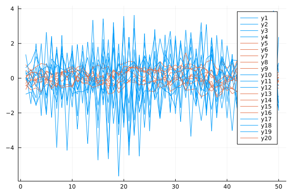
We generate a 10 time series of 50 point using the two above models parameters. The model parameters are slightly perturbed for producing a time series with uniques model properties.
Variables:
- $k$ is a number of models
- $n$ is a size of a time series
- $m$ is a number of time series for a particular model
using ARFIMA, Random, Statistics
k, n, m, α = 2, 50, 10, 0.05
rng = MersenneTwister(1)
ϵ = α*randn(m,p+q)
C1 = hcat((arma(rng, n, σ₁²[], SVector(ϕ₁.+ϵ[i,1:2]...), SVector(θ₁.+ϵ[i,3]...)) for i in 1:m)...)
C2 = hcat((arma(rng, n, σ₂²[], SVector(ϕ₂.+ϵ[i,1:2]...), SVector(θ₂.+ϵ[i,3]...)) for i in 1:m)...)
# combine data and shuffle dataset
rng = MersenneTwister(1)
X = [C1 C2][:,shuffle(rng, 1:2m)];
using Plots
ORIG = ARMAMixtureModel([ARMA(ϕ₁, θ₁, σ₁²[]); ARMA(ϕ₂, θ₂, σ₂²[])], [0.5, 0.5])
@show ORIG
prediction = predict(ORIG,X,typ=:hard)
@show prediction
@show counts(prediction)
plot(X, c=[i for j in 1:n, i in prediction])
ORIG = Mixture Model{ARMA{Float64}}(K = 2)
components[1] (prior = 0.5): ARMA: ϕ=[-0.05, 0.82], θ=[0.44], σ²=0.86
components[2] (prior = 0.5): ARMA: ϕ=[0.34, 0.27], θ=[-0.25], σ²=0.34
prediction = [1, 1, 1, 1, 2, 2, 2, 2, 2, 1, 1, 1, 2, 2, 2, 2, 1, 1, 1, 2]
counts(prediction) = [10, 10]
The ARMA($p$, $q$) refers to the model with $p$ autoregressive terms and $q$ moving-average terms. This model contains the AR($p$) and MA($q$) models,
\begin{equation}\label{eq:arma} x_{t} = c + \varepsilon_{t}+\sum_{i=1}^{p}\varphi_{i}X_{t-i}+\sum_{i=1}^{q}\theta_{i}\varepsilon_{t-i} \end{equation}
The logarithm of the conditional likelihood function of the ARMA model is \begin{equation}\label{eq:arma-lekelihood} \ln p(\boldsymbol z|\boldsymbol \Phi) = -\frac{n}{2}\ln(2\pi\sigma^2) - \frac{1}{2\sigma^2}\sum_{t=1}^{n} e_t^2 \end{equation}
where $\boldsymbol \Phi = { \boldsymbol \varphi, \boldsymbol \theta, \sigma^2}$ is the $p + q + 1$ parameters of the ARMA model, and $e_t$ is estimated recursively, such that
$$e_t = x_t - c - \sum_{j=1}^p \varphi_j x_{t-j} - \sum_{j=1}^{q}\theta_{j}e_{t-i}$$
Now we need to define a likelihood function for ARMA mixture [4]. We write it in a log form as follows:
\begin{equation} \label{eq:arma-mix} \ln p(\boldsymbol x | \boldsymbol \Theta) = \ln \sum_{i=1}^{k} \pi_i(\boldsymbol q) p(\boldsymbol x | \boldsymbol \Phi_i) \end{equation}
where $\boldsymbol \Theta = {\boldsymbol \Phi_1, \ldots, \Phi_k, \boldsymbol q}$. We use reparametrized prior $\pi_i(\boldsymbol q)$ as in \eqref{eq:prior-reparam} to ensure probability unit constraint.
The implementation of the log-likelihood for the ARMA model was shown in the previous blog post on MLE optimization for regression models.
The ARMA mixture log-likelihood defined through the sum of log prior and log-likelihood of a specific ARMA model, and logsumexp function for the numerical stability as follows:
\begin{equation} \label{eq:arma-mix2} \ln p(\boldsymbol x | \boldsymbol \Theta) = \ln \sum_{i=1}^{k} \exp\left( \ln\pi_i(\boldsymbol q) + \ln p(\boldsymbol x | \boldsymbol \Phi_i) \right) \end{equation}
In addition, we also need to write a some auxiliary functions for (un)packing parameters into a one-dimensional vector, for compatibility with the function representation required for automatic differentiation in ForwardDiff.jl package.
function loglikelihood(Φ, conf, X)
    ϕs, θs, σs, πs, k = unpack(Φ, conf)
    res = 0
    for x in eachcol(X)
        ps = [ log(πs[i]) + loglikelihood(x, ϕs[i], θs[i], σs[i]) for i in 1:k ]
        res += logsumexp(ps)
    end
    res
end
# test ARMA mixture log-likelihood
let conf = (p,q), # ARMA(2,1)
    Φ = pack([ϕ₁, ϕ₂], [θ₁, θ₂], [σ₁², σ₂²], [1.0])
    loglikelihood(Φ, conf, X)
end
-1133.1585520307406
Now, we are ready for the optimization. We use LBFGS optimizer to find a minimum of the ARMA mixture negative log-likelihood function. The initial model parameters are randomized/zerod.
using Optim
Random.seed!(1)
res = let conf = (p,q), # ARMA(2,1)
    k = 2,
    ϕs = [zeros(p) for i in 1:k],
    θs = [rand(q) for i in 1:k],
    σs = ones(k),
    qs = rand(k-1),
    Φ0 = pack(ϕs, θs, σs, qs)

    @show Φ0
    optimize(Φ->-loglikelihood(Φ, conf, X), Φ0, LBFGS(); autodiff = :forward)
end
Φ0 = [0.0, 0.0, 0.0, 0.0, 0.23603334566204692, 0.34651701419196046, 1.0, 1.0, 0.3127069683360675]

 * Status: success

 * Candidate solution
    Final objective value:     8.063637e+02

 * Found with
    Algorithm:     L-BFGS

 * Convergence measures
    |x - x'|               = 1.64e-11 ≰ 0.0e+00
    |x - x'|/|x'|          = 1.64e-11 ≰ 0.0e+00
    |f(x) - f(x')|         = 1.14e-13 ≰ 0.0e+00
    |f(x) - f(x')|/|f(x')| = 1.41e-16 ≰ 0.0e+00
    |g(x)|                 = 2.10e-11 ≤ 1.0e-08

 * Work counters
    Seconds run:   0  (vs limit Inf)
    Iterations:    33
    f(x) calls:    101
    ∇f(x) calls:   101
We define a “hard” probabilistic classifier that allow as partition our dataset, and see from which component of the mixture a point is originated.
OPT = build_model(unpack(Optim.minimizer(res), (p,q))...)
@show OPT
prediction = predict(OPT,X,typ=:hard)
@show prediction
@show counts(prediction)
plot(X, c=[i for j in 1:n, i in prediction])
OPT = Mixture Model{ARMA{Float64}}(K = 2)
components[1] (prior = 0.5000000000027094): ARMA: ϕ=[0.03631141443150687, 0.8435028164320373], θ=[-0.5070982975148999], σ²=0.741953670786134
components[2] (prior = 0.4999999999972906): ARMA: ϕ=[0.4647442432042342, 0.2402270819875525], θ=[0.0470466065015753], σ²=0.1099991464094101
prediction = [1, 1, 1, 1, 2, 2, 2, 2, 2, 1, 1, 1, 2, 2, 2, 2, 1, 1, 1, 2]
counts(prediction) = [10, 10]

We find two clusters of time series in the dataset which correspond to the original classes in the given dataset.
References
[1] Bishop, Christopher M. Pattern Recognition and Machine Learning. Information science and statistics. Springer, Heidelberg, 2006.
[2] Box, George EP, Gwilym M. Jenkins, Gregory C. Reinsel, and Greta M. Ljung. Time series analysis: forecasting and control. John Wiley & Sons, 2015.
[3] Alexandrovich, Grigory. An exact Newton’s method for ML estimation of a Gaussian mixture. 2014.
[4] Xiong, Yimin, and Dit-Yan Yeung. Time series clustering with ARMA mixtures. Pattern Recognition 37.8, 2004: 1675-1689.