Introduction
The goal of regression is to predict the value of one or more continuous target variables $t$ given the value of a $D$-dimensional vector $x$ of input variables. The polynomial is a specific example of a broad class of functions called linear regression models. The simplest form of linear regression models are also linear functions of the input variables. However, much more useful class of functions can be constructed by taking linear combinations of a fix set of nonlinear functions of the input variables, known as basis functions [1].
Regression models can be used for time series modeling. Typically, a regression model provides a projection from the baseline status to some relevant demographic variables. Curve-type time series data are quite common examples of these kinds of variables. Typical time series model is the ARMA model. It’s a combination of two types of time series data processes, namely, autoregressive and moving average processes.
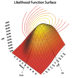
Both, regression and time series models uses maximum likelihood estimation optimization for finding optimal parameters of the model. This likelihood principle says that, given that the assumed model is correct, all that the data have to tell us about the parameters is contained in the likelihood function, all other aspects of the data being irrelevant. From a Bayesian point of view, the likelihood function is equally important, since it is the component in the posterior distribution of the parameters that comes from the data [2].
Basis Function Models
Often times we want to model data $y$ that emerges from some underlying function $f(x)$ of independent variables $x$ such that for some future input we’ll be able to accurately predict the future output values. There are various methods for devising such a model, all of which make particular assumptions about the types of functions the model can emulate. In this post we’ll focus on one set of methods called Basis Function Models (BFMs).
There is a class of models represented by linear combinations of fixed nonlinear functions of the input variables, of the form
\begin{equation} y(\boldsymbol x, \boldsymbol w) = \sum^{M-1}_{j=0} w_j\phi_i(\boldsymbol x) = \boldsymbol w^T \boldsymbol \phi(\boldsymbol x) \end{equation}
where $\boldsymbol w = (w_0, \ldots, w_{M-1})^T$ and $\boldsymbol \phi = (\phi_0, \ldots, \phi_{M-1})^T$ [1].
- It is often convenient to define an additional dummy basis function $\phi_0(\boldsymbol x) = 1$.
- Basis functions are also sometimes called kernels.
Naturally, we would define this function in Julia as
y(x::Real, w; ϕ=ϕ) = w'ϕ(x)
y (generic function with 1 method)
but we also might need more efficient broadcast version for $N$-dimensional input is
y(xs, w; ϕ=ϕ) = [w'].*(ϕ.(xs)) # broadcasted w'ϕ(x)
y (generic function with 2 methods)
We initialize some auxiliary packages for plotting and random number generation
using Plots  # plotting
using Flux   # ML / AD
using Random # RNG
default(fmt = :png)
and generate some random weights for our example models.
Random.seed!(1)
d, n = 3, 5
xs = -5.0:0.1:5
@show xs
ws = randn(d,n)
xs = -5.0:0.1:5.0

3×5 Matrix{Float64}:
  0.297288  -0.0104452  2.29509   -2.26709   0.583708
  0.382396  -0.839027   0.408396   0.529966  0.963272
 -0.597634   0.311111   0.22901    0.431422  0.458791
Let’s take a look at examples of basis function models for creating a some data trends.
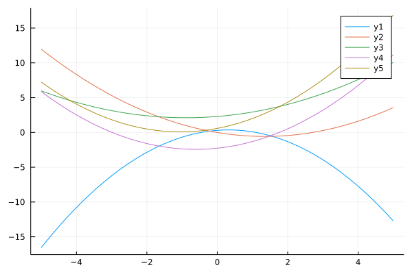
We start with polynomial basis: $\phi_j(x) = x^j$.
ϕ_p(x;p=2) = [x^p for p in 0:p]
@show ϕ_p(3);
ϕ_p(3) = [1, 3, 9]
ys = mapslices(w->y(xs, w; ϕ=ϕ_p), ws, dims=1)
plot(xs, ys)
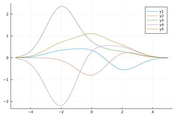
Very common BFM is a Gaussian kernel function: $\phi(\boldsymbol x) = \exp\left\lbrace -\frac{||\boldsymbol x- \boldsymbol \mu||_2^2}{2\sigma^2}\right \rbrace$. We define it for 1D case as follows:
ϕ_g(x; μs, σ²=1.0) = [ exp(-(x-μ)^2/(2σ²)) for μ in μs]
@show ϕ_g(1;μs=rand(2));
ϕ_g(1; μs = rand(2)) = [0.6188869235931157, 0.7759365188062989]
μs = [-2.0, 0.0, 2.0] # various Gaussian means
@show μs
ys = mapslices(w->y(xs, w; ϕ=x->ϕ_g(x;μs)), ws, dims=1)
plot(xs, ys)
μs = [-2.0, 0.0, 2.0]
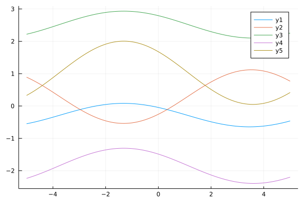
Another option for basis functions, particularly for periodic data, is the Fourier basis. One straightforward approach is to choose a set of frequencies and phases and construct the basis as in: $\phi_0(x) = 1$, $\phi_j(x) = cos(\omega_j x + \psi_j)$
ϕ_ft(x;ωs,ψs) = [1; cos.(ωs*x+ψs)]
@show ϕ_ft(5;ωs=rand(3),ψs=rand(3));
ϕ_ft(5; ωs = rand(3), ψs = rand(3)) = [1.0, 0.442797057781095, 0.787941955488779, -0.6882652718378672]
ωs=rand(2)
ψs=rand(2)
ys = mapslices(w->y(xs, w; ϕ=x->ϕ_ft(x;ωs,ψs)), ws, dims=1)
plot(xs, ys)
Maximum Likelihood Estimation
The coefficients values, $\boldsymbol w$, are obtained by fitting $y(\boldsymbol x, \boldsymbol w)$ to training data $t$:
- We assume that the target variable t is given by a deterministic function $y(\boldsymbol x, \boldsymbol w)$ with additive Gaussian noise so that $$t = y(\boldsymbol x, \boldsymbol w) + \epsilon$$
where $\epsilon$ is a zero mean Gaussian random variable with precision (inverse variance), $\beta^{-1} = \sigma^2$.
Thus, a model of the above linear model for regression is
$$p(t|\boldsymbol x, \boldsymbol w, \beta) = \mathcal{N}(t|y(\boldsymbol x, \boldsymbol w), \beta^{-1})$$
By minimizing an error function, a measure of misfit between function $y(\boldsymbol x, \boldsymbol w)$ for any given value of $\boldsymbol w$, and the training set data points $\boldsymbol t$.
- A choice of error function is the sum of the squares of the errors between predictions $y(\boldsymbol x_i, \boldsymbol w)$ for each point $\boldsymbol x_i$ and corresponding target values $t_i$
\begin{equation}\label{eq:error-comp} E(\boldsymbol w) = \frac{1}{2} \sum_{i=1}^{N}(t_i - y(\boldsymbol x_i, \boldsymbol w)))^2 = \frac{1}{2} \sum_{i=1}^{N}(t_i - \boldsymbol w^T \boldsymbol \phi(\boldsymbol x_i))^2 \end{equation}
 |
| Image source |
The likelihood function of the conditional distribution $p(t|\boldsymbol x, \boldsymbol w, \beta)$ is
$$p(\boldsymbol t|\boldsymbol x, \boldsymbol w, \beta) = \prod_{i=1}^{N} \mathcal{N}(t|\boldsymbol w^T \boldsymbol \phi(\boldsymbol x_i), \beta^{-1})$$
And its logarithm is
\begin{equation}\label{eq:log-likelihood} \ln p(\boldsymbol t|\boldsymbol x, \boldsymbol w, \beta) = \sum_{i=1}^{N} \ln \mathcal{N}(t|\boldsymbol w^T \boldsymbol \phi(\boldsymbol x_i), \beta^{-1}) = \frac{N}{2}\ln\beta - \frac{N}{2}\ln(2\pi) - E(\boldsymbol w) \end{equation}
In order to find parameters of a linear basis function model, $p(\boldsymbol t|\boldsymbol x, \boldsymbol w, \beta)$, we maximize likelihood or minimizing the negative log likelihood with respect to $\boldsymbol w$:
$$\arg\min_{\boldsymbol w, \beta} -\ln p(\boldsymbol t|\boldsymbol x, \boldsymbol w, \beta)$$
Maximization of the likelihood function under a conditional Gaussian noise distribution for a linear model is equivalent to minimizing a sum-of-squares error function given by $E(\boldsymbol w)$.
BFM Fitting
Instead of finding a solution in a closed form, we’ll optimize our likelihood function using stochastic gradient descent (SGD) algorithm accompanied with automatic differentiation for calculation of the gradient of error function, $\nabla E(\boldsymbol w)$. For this exercise, we only consider finding optimal weights and disregard precision parameter.
Polynomial Basis Functions
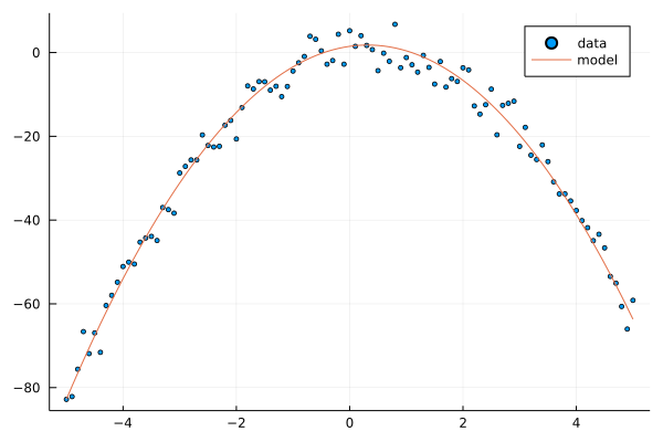
We begin with example of polynomial BFM. Given model weights, we generate noisy data from the model.
Random.seed!(1)
xs = -5:0.1:5; @show xs;
w = 5*randn(3); @show w; # model weight
ts = y(xs, w; ϕ=ϕ_p) .+ 3*randn(length(xs)); # our dataset
scatter(xs, ts, label="data", ms=2.5)
plot!(xs, y(xs, w; ϕ=ϕ_p), label="model")
xs = -5.0:0.1:5.0
w = [1.4864399226773082, 1.9119798389530391, -2.988172383641156]
We’ll use Flux machine learning library that provides automatic differentiation and optimization components.
First, we define a variable w_p for keeping model weights, a loss function as in $\eqref{eq:error-comp}$.
Random.seed!(42)
w_fit = randn(3)
loss(x, t) = sum((t .- y(x, w_fit; ϕ=ϕ_p)).^2)
loss(xs, ts)
113890.83738980447
We perform mini-batch SGD optimization for finding the weight of our BF model. For that we need to setup a DataLoader object that allows to batch and shuffle data for SGD optimizer. Then, we initialize optimizer and parameters object for optimization.
# use data wrapper for batching and shuffling
data = Flux.Data.DataLoader((xs, ts); batchsize=1, shuffle=true)
opt = ADAM()   # optimizer
θ = params(w_fit) # optimized model parameters
for i in 1:300
    Flux.train!(loss, θ, data, opt)
    i % 100 == 0 && println("Iteration $i: loss=", loss(xs, ts))
end
Iteration 100: loss=1402.566728293691
Iteration 200: loss=971.2551022387617
Iteration 300: loss=939.0477624922326
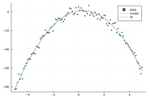
Here is an original and fitted weights of the model, and figure of how models are related to the dataset.
@show w
@show w_fit;
scatter(xs, ts, label="data", ms=2.5)
plot!(xs, y(xs, w; ϕ=ϕ_p), label="model")
plot!(xs, y(xs, w_fit; ϕ=ϕ_p), label="fit")
w = [1.4864399226773082, 1.9119798389530391, -2.988172383641156]
w_fit = [0.5637108579574772, 1.984690247289546, -2.9091503333715]
Gaussian Basis Functions
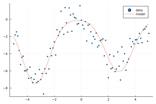
In the second example, we use Gaussian BFM. Similar to the previous example, we generate random weights for the model, and then a dataset from noisy model observations.
Random.seed!(2)
w = 10*randn(3); @show w;  # weights
μs = 5*randn(3); @show μs; # Gaussian means
ts = y(xs, w; ϕ=x->ϕ_g(x;μs)) .+ randn(length(xs)); # model + noise
scatter(xs, ts, label="data", ms=2.5)
plot!(xs, y(xs, w; ϕ=x->ϕ_g(x;μs)), label="model")
w = [7.396206598864331, -7.445071021408705, -6.085075626113596]
μs = [-8.617282553978992, -3.378078037011857, 2.7832316668506536]
Now, we optimize the SSE loss function with respect to the model weights, and also with respect to Gaussian means which are additional parameters of our model.
Random.seed!(42)
w_fit = randn(3)
μ_fit = randn(3)
# loss(x, t) = sum((y(x, w_fit; ϕ=x->ϕ_g(x;μs)) .- t).^2) # w only
loss(x, t) = sum((y(x, w_fit; ϕ=x->ϕ_g(x;μs=μ_fit)) .- t).^2) # w + μ
# λ = 0.1; loss(x, t) = sum((y(x, w_fit; ϕ=x->ϕ_g(x;μs=μ_fit)) .- t).^2) + λ*(w_fit'w_fit)/2 # w + μ regularized
loss(xs, ts)
1535.0508737251694
opt = ADAM()
# θ = params(w_fit) # w only
θ = params(w_fit, μ_fit) # w + μ
data = Flux.Data.DataLoader((xs, ts); batchsize=1, shuffle=true)
for i in 1:300
    Flux.train!(loss, θ, data, opt)
    i % 100 == 0 && println("Iteration $i: loss=", loss(xs, ts))
end
Iteration 100: loss=220.98028454191237
Iteration 200: loss=89.17856789448327
Iteration 300: loss=88.9463229717334
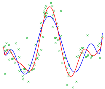
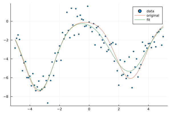
Despite slow convergence, the fitted model behaves relatively well in comparison to the original model given the nosiness of the dataset.
scatter(xs, ts, label="data", ms=2.5)
plot!(xs, y(xs, w; ϕ=x->ϕ_g(x;μs)), label="original")
# plot!(xs, y(xs, w_fit; ϕ=x->ϕ_g(x;μs=μs)), label="fit")  # w only
plot!(xs, y(xs, w_fit; ϕ=x->ϕ_g(x;μs=μ_fit)), label="fit") # w + μ
ARMA
Another common model for fitting time series data is Autoregressive–moving-average model (ARMA). The notation ARMA($p$, $q$) refers to the model with $p$ autoregressive terms and $q$ moving-average terms. This model contains the AR($p$) and MA($q$) models,
\begin{equation}\label{eq:arma} x_{t} = c + \varepsilon_{t}+\sum_{i=1}^{p}\varphi_{i}X_{t-i}+\sum_{i=1}^{q}\theta_{i}\varepsilon_{t-i} \end{equation}
where $\varphi_{1},\ldots ,\varphi_{p}, \theta_1, \ldots, \theta_q$ are the parameters of the model, the set of AR($p$) and MA($q$) coefficient, $c$ is a constant, and the random variable $\varepsilon _{t}$ is white noise with variance $\sigma^2$ [2].
Suppose that we have a sample of an $N$-dimensional random variable $\boldsymbol z$, whose known probability distribution $p(\boldsymbol z|\boldsymbol \Phi)$ depends on some unknown set of parameters $\boldsymbol \Phi$. In particular, this set could refer to the $p + q + 1$ parameters $\boldsymbol \Phi = { \boldsymbol \varphi, \boldsymbol \theta, \sigma^2}$ of the ARMA model.
We can express the natural logarithm of the conditional likelihood function as \begin{equation}\label{eq:arma-lekelihood} \ln p(\boldsymbol z|\boldsymbol \Phi) = -\frac{n}{2}\ln(2\pi\sigma^2) - \frac{1}{2\sigma^2}\sum_{t=1}^{n} e_t^2 \end{equation}
where $e_t$ must be estimated recursively, such that
$$e_t = x_t - c - \sum_{j=1}^p \varphi_j x_{t-j} - \sum_{j=1}^{q}\theta_{j}e_{t-i}$$
ARMA Fitting
using ARFIMA
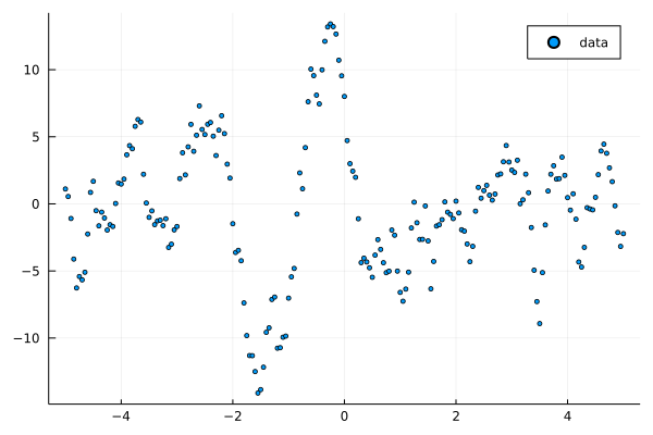
Random.seed!(2)
σ, φ, θ = 1.5, 0.9, 0.6
xs = -5:0.05:5
N = length(xs)
ts = arma(length(xs), σ, SVector(φ), SVector(-θ));
scatter(xs, ts, label="data", ms=2.5)
Because ARMA likelihood calculations has recursive component, the previous values of errors, see $\eqref{eq:arma-lekelihood}$, we need to keep a history of all calculated errors during the calculation. Thus, we define a dictionary structure hist for keeping previosly computed.
function loglkhd(xs::Vector{T}, φs::Vector{T}, θs::Vector{T}, σ²::Vector{T};
                 hist=Dict(0=>zero(T))) where T
    n = length(xs)
    p, q = length(φs), length(θs)
    total = zero(T)
    @inbounds for t in 1:n
        s = zero(T)
        for j in 1:p # AR
            if t-j > 0
                s += φs[j]*xs[t-j]
            end
        end
        for j in 1:q # MA
            if t-j > 0
                s += θs[j]*hist[t-j]
            end
        end
        err = xs[t] - s
        hist[t] = err
        total += err^2
    end

    -(n*log(2π*σ²[])/2 + total/(2σ²[]))
end
loglkhd (generic function with 1 method)
Here is a log-likelihood value for original model parameter.
loglkhd(ts, [φ], [θ], [σ^2])
-361.1361626447399
Our optimization minimized the negative log-likelihood of ARMA model. Using Flux training loop structure as an example of the simple AD optimizer.
function sgd!(φs, θs, σ², ts, opt; iter=10)
    prms = params(φs, θs, σ²)
    for i in 1:iter
        grads = gradient(prms) do
            -loglkhd(ts, φs, θs, σ²)
        end
        for p in prms
            Flux.Optimise.update!(opt, p, grads[p])
        end
    end
    prms
end
sgd! (generic function with 1 method)
We start with unit variance and “white” noise parameters, i.e. ARMA parameters are set to zero value.
φ_fit, θ_fit, σ²_fit = zeros(1), zeros(1), ones(1)
opt = ADAM(0.1)
@time sgd!(φ_fit, θ_fit, σ²_fit, ts, opt; iter=100)
@show φ_fit
@show θ_fit
@show √σ²_fit[];
@show loglkhd(ts, φ_fit, θ_fit, σ²_fit);
  8.914507 seconds (11.02 M allocations: 655.491 MiB, 6.04% gc time, 95.23% compilation time)
φ_fit = [0.9049125062520333]
θ_fit = [0.5985401118231235]
√(σ²_fit[]) = 1.4842023218438392
loglkhd(ts, φ_fit, θ_fit, σ²_fit) = -361.05867523532993
The fitted model parameters are very close to the original parameters. If we compare results to parameters from R package artfima, we find our results are better fitted.
using RCall
@rlibrary artfima
res = artfima(ts, arimaOrder = [1, 0, 1])
φ_R, θ_R, σ²_R = res[3][],-res[4][],res[6][]
@show loglkhd(ts, [φ_R], [θ_R], [σ²_R])
res
loglkhd(ts, [φ_R], [θ_R], [σ²_R]) = -361.2216469662469

RObject{VecSxp}
ARTFIMA(1,0,1), MLE Algorithm: exact, optim: BFGS
snr = 11.756, sigmaSq = 2.11392525246811
log-likelihood = -361.9, AIC = 735.8, BIC = 755.62
                est.   se(est.)
mean     -0.35425468 0.51721049
d         0.04521304 0.11828350
lambda    0.12670577 0.31545090
phi(1)    0.88099629 0.04883283
theta(1) -0.58730731 0.07647501
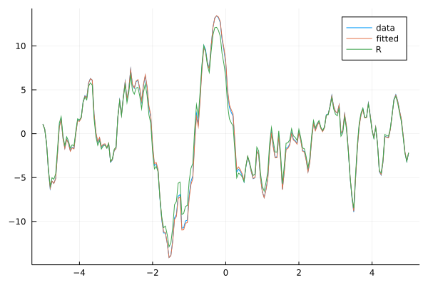
Graphically our fitted model is indistinguishable from the original one.
plot(xs, ts, label="data")
Random.seed!(2)
ts_fit = arma(N, sqrt(σ²_fit[]), SVector(φ_fit[]), SVector(-θ_fit[]));
plot!(xs, ts_fit, label="fitted")
Random.seed!(2)
ts_R = arma(N, sqrt(σ²_R), SVector(φ_R), SVector(-θ_R));
plot!(xs, ts_R, label="R")
Conclusion
We showed that automatic differentiation is a powerful tool that allows quickly define simple routine for MLE optimization without complex programming associated with an implementation of a close form solutions. The AD-driven optimizations showed similar accuracy to well known method for regression and time series model fitting.
References
[1] Bishop, Christopher M. Pattern Recognition and Machine Learning. Information science and statistics. Springer, Heidelberg, 2006.
[2] Box, George EP, Gwilym M. Jenkins, Gregory C. Reinsel, and Greta M. Ljung. Time series analysis: forecasting and control. John Wiley & Sons, 2015.