Nonlinear Dimensionality Reduction

In statistical learning, many problems require initial preprocessing of multi-dimensional data, and often reduce dimensionality of the data, in a way, to compress features without loosing information about relevant data properties. Common linear dimensionality reduction methods, such as PCA or MDS, in many cases cannot properly reduce data dimensionality especially when data located around nonlinear manifold embedding in high-dimensional space.

There are many nonlinear dimensionality reduction (NLDR) methods for construction of low-dimensional manifold embeddings. A Julia language package ManifoldLearning.jl provides implementation of most common algorithms.

Manifold Learning

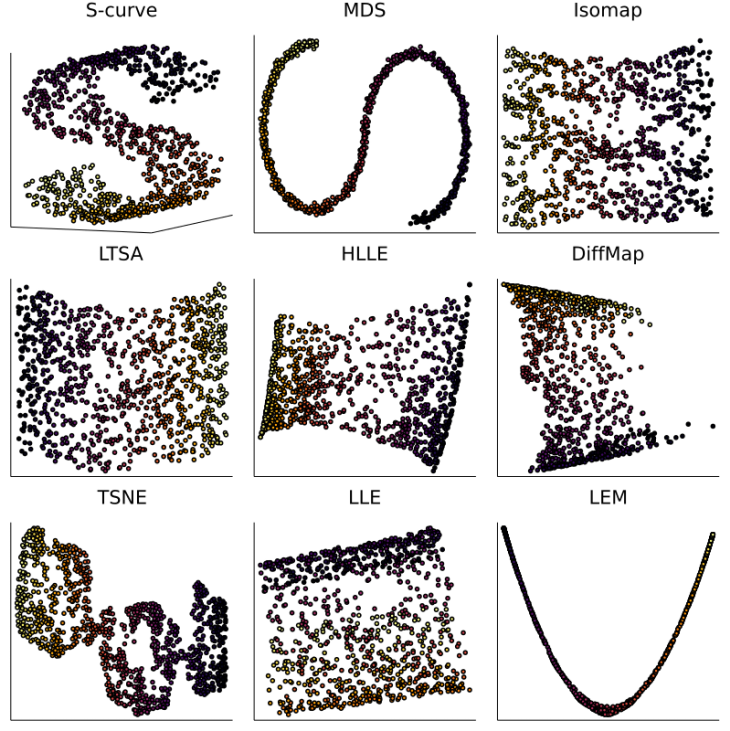
A comparison of various dimensionality reduction methods form ManifoldLearning.jl on a common synthetic dataset, S-curve.

using ManifoldLearning, StableRNGs, Plots
default(fmt = :png)

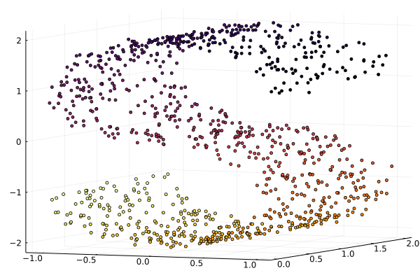
The ManifoldLearning.jl package provide several synthetic datasets for testing purposes. We generate the S-curve dataset composed of 1000 points.

rng = StableRNG(42)
X, L = ManifoldLearning.scurve(rng=rng, segments=0)
size(X)

(3, 1000)

scatter3d(X[1,:], X[2,:], X[3,:], zcolor=L, palette=cgrad(:jet1), ms=2.5, leg=:none, camera=(30,15))

png

ManifoldLearning.jl package provides API similar to various packages from JuliaStats organization: fit function, that performs model fitting given the sample data, and predict function, that returns a data low-dimensional embedding.

Let’s define common parameters for the reduction procedure. Many manifold learning algorithm rely on nearest neighbor graph of data points for approximation of the local manifold neighborhood around the data point, $k$.

d = 2 # an embedding dimension
k = 12 # a number nearest neighbors for approximation

The data has to be in column-major format, each column corresponds to a sample/observation, while each row corresponds to a feature (variable or attribute), when it’s passed to fit method call.

M = fit(Isomap, X, k=k, maxoutdim=d)

Isomap{BruteForce}(indim = 3, outdim = 2, neighbors = 12)

The result of the fit call is a particular NLDR model which can be used for data transformation. By default, a distance matrix is used for searching $k$-nearest neighbors (BruteForce type). This default approach is acceptable for small datasets, because its time and space complexity is $O(n^2)$, and can cause significant slowdown for large datasets. Use plug-in wrappers for KD-tree implementations from NearestNeighbors.jl or FLANN.jl to speed up computations for large datasets.

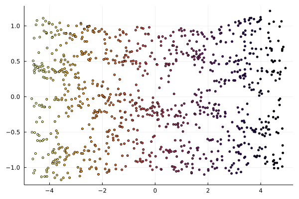
The predict method call returns a data embedding given a particular NLDR model.

Y = predict(M)
size(Y)

(2, 1000)

Following picture shows an “unrolled” S-curve as a 2D embedding of the original 3D dataset.

scatter(Y[1,:], Y[2,:], zcolor=L, palette=cgrad(:jet1), ms=2.5, leg=:none)

png

Algorithm Comparison

Now, we compare multiple NLDR dimensionality methods on the above dataset, as well as linear dimensionality reduction methods, s.t. PCA or MDS (from MultivariateStats.jl package).

Fitting linear models:

using MultivariateStats
M_mds = fit(MDS, X, maxoutdim=d, distances=false)

MDS{Float64}

Fitting nonlinear models:

nldr = [Isomap, LEM, LLE, LTSA]
nlinmodels = [
    [fit(alg, X, maxoutdim=d, k=k) for alg in nldr];
    fit(HLLE, X, k=2k, maxoutdim=d);
    fit(DiffMap, X, α=0.5, maxoutdim=d);
    fit(TSNE, X, maxoutdim=d, p=60)
]

7-element Vector{MultivariateStats.NonlinearDimensionalityReduction}:
 Isomap{BruteForce}(indim = 3, outdim = 2, neighbors = 12)
 LEM{BruteForce}(indim = 3, outdim = 2, neighbors = 12)
 LLE{BruteForce}(indim = 3, outdim = 2, neighbors = 12)
 LTSA{BruteForce}(indim = 3, outdim = 2, neighbors = 12)
 HLLE{BruteForce}(indim = 3, outdim = 2, neighbors = 24)
 Diffusion Maps(indim = 3, outdim = 2, t = 1, α = 0.5, ɛ = 1.0)
 t-SNE{BruteForce}(indim = 3, outdim = 2, perplexity = 60)

By calling predict, we obtain a low-dimensional embedding of the dataset.

Ys = Dict(string(mn)=>predict(md) for (mn, md) in zip(
            [MDS; nldr; HLLE; DiffMap; TSNE], [M_mds; nlinmodels]
        ))

Dict{String, AbstractMatrix{Float64}} with 8 entries:
  "MDS"     => [-0.245604 2.03335 … -0.447666 1.71374; -0.690183 0.0416312 … -0…
  "Isomap"  => [-0.649127 3.17315 … -0.867408 2.42836; 0.39137 -0.21987 … -0.04…
  "LTSA"    => [0.00830175 -0.0365208 … 0.0113566 -0.0289106; 0.00992206 -0.001…
  "HLLE"    => [-0.560897 1.22124 … -0.600436 0.984536; -0.381499 -0.108029 … 0…
  "DiffMap" => [-0.0329479 -0.0325822 … -0.0345897 -0.0333053; 0.0107813 -0.041…
  "TSNE"    => [-5.77682 30.258 … -6.51834 20.658; -0.592248 -0.230137 … -2.605…
  "LLE"     => [0.770951 -0.309381 … 0.231706 0.0198379; -0.640712 1.26445 … -0…
  "LEM"     => [0.00204649 -0.010625 … 0.00289824 -0.00883087; -0.0119373 0.006…

Now, plotting all results on one screen. Note that MDS fail to unroll the curved manifold structure.

plotparams = [:zcolor=>L, :ms=>2.3, :ticks=>nothing, :leg=>:none]
Ps = [scatter(Y[1,:], Y[2,:]; title=n, plotparams...) for (n,Y) in Ys];
pushfirst!(Ps, scatter3d(X[1,:], X[2,:], X[3,:]; camera=(30,15), title="S-curve", plotparams...))
plot(Ps..., size=(800,800))

png