Introduction
Stochastic gradient descent (SGD) is a popular stochastic optimization algorithm in the field of machine learning, especially for optimizing deep neural networks. In its core, this iterative algorithm combines two optimization techniques: a stochastic approximation with gradient descent.
SGD is common for optimizing various range of models. We are interested in application of this optimization techniques to standard data science tasks as linear regression and clustering. In addition, we’ll use differentiable programming techniques for simplifying and making versatile our SGD implementation.
Linear Regression
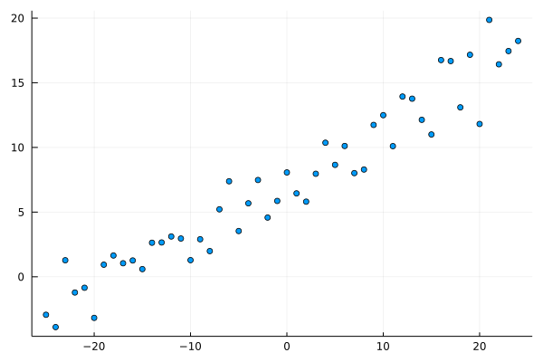
Our first task is a linear regression problem. Let’s generate a dataset.
using Random, LinearAlgebra, Statistics
function dataset(n = 50; trend=true)
    x = reshape(range(-n/2, length=n), n, 1) |> collect
    m = rand(n).*0.2.+0.3
    b = rand(n).*5 .+ 5
    y = trend ? m.*x .+b : rand(n).*20 .- 10
    x, vec(y)
end
dataset (generic function with 2 methods)
using Random, Plots
default(fmt = :png)
Random.seed!(42);
n = 50
x, y = dataset(n)
scatter(x, y; leg=:none)
A simple 1D linear regression model is defined as follows
$$\hat{y} = \beta_0 + \beta_1 x + \varepsilon$$
or in matrix notation
$$ \hat{\mathbf{y}} =\mathrm {X} {\boldsymbol {\beta }}+{\boldsymbol {\varepsilon }} $$
We’ll define a corresponding lr_model function which represents this linear model:
lr_model(w, x) = w[1] .+ x.*w[2]
lr_model (generic function with 1 method)
OLS solution
Our goal is to find a parameters of our linear regression model, $\boldsymbol{\beta }$. The solution for can be defined in closed form
$$\hat{\boldsymbol {\beta }}=\left(\mathrm {X} ^{\mathsf {T}}\mathrm {X} \right)^{-1}\mathrm {X} ^{\mathsf {T}}\mathbf {y}$$
It is derived from the quadratic minimization problem of the ordinary least squares (OLS),
$$\hat{\boldsymbol {\beta }} = \arg\min_{\boldsymbol{\beta }} S({\boldsymbol{\beta }})$$
where $S({\boldsymbol{\beta }})= {\bigl |}\mathbf {y} -\mathrm {X} {\boldsymbol {\beta }}{\bigr |}^{2}$.
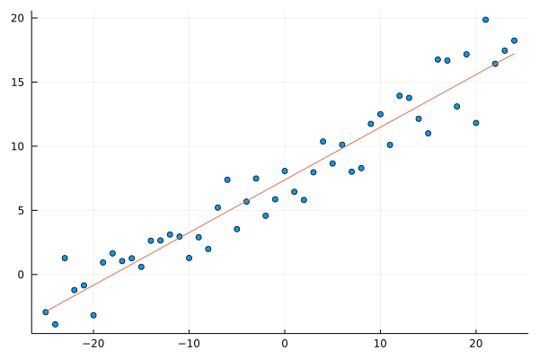
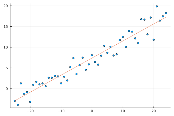
Let’s compute and plot the solution.
X = hcat(ones(n), x)
β = inv(X'X)*X'y
2-element Vector{Float64}:
 7.372660709945862
 0.41063191822595657
scatter(x, y; leg=:none)
plot!(x, lr_model(β,x))
SGD solution
We start with a basic implementation of the SGD algorithm using automatic differentiation.
Now, we need to define a loss function for evaluating our regression model. Let’s pick the mean square error (MSE), $$MSE(\beta) = \frac{1}{n}\sum_{i=1}^{n}(y_i - \hat{y_i})^2$$
# MSE loss function
loss(y,ŷ) = mean((y.-ŷ).^2)
# Let's test it
loss(y, lr_model(β, x))
2.802066067141918
The standard gradient descent algorithm that is used for minimizing loss functions with the form of a sum
$$Q(w) = \sum_{i=1}^n Q_i(w)$$
Using the standard gradient descent algorithm, $Q$ can be minimized by the iteration
$$w_{t+1} = w_{t} - \eta \nabla Q(w_t) $$ $$ = w_{t} - \eta \nabla \sum_{i=1}^n Q_i(w_t) $$
where $\eta>0$ is a step size.
In the stochastic gradient descent, $Q$ is minimized using
$$ w_{t+1} = w_{t} - \eta \nabla Q_i(w_t) $$
updating the weights $w$ in each step using just one sample $i$ randomly chosen from the dataset.
The close form gradient of the MSE with respect to $\beta$ (see above OLS solution) is
$$ \nabla MSE(\beta) = \frac{2}{n}(X’X \boldsymbol\beta - X’y) $$
However, we’ll use automatic differentiation, ForwardDiff.jl package, to compute numerically this gradient in the SGD optimization problem setup.
Let’s define an SGD iteration using automatic differentiation which includes
- iteration limit
- convergence rate
- mini-batch size
using ForwardDiff: gradient

function sgd!(w, f, xs, ys=zeros(size(xs,1)); η=0.01, ε=0.01, maxiter=100, batch=1, skip=0)
    n = size(xs,1)
    batch = min(batch, n)
    i = 1
    while i < maxiter # iteration termination
        # sample mini-batch
        idxs = rand(1:n, batch)
        sample_x, sample_y = view(xs, idxs, :), view(ys, idxs)
        # determine parameter's gradient
        ∇w = gradient(w->loss(sample_y, f(w, sample_x)), w)
        # check for the convergence rate
        norm(∇w) < ε && break
        # update parameters
        w .-= η*∇w
        # debugging
        if skip > 0 && i%skip == 0
            println("Itr: $i, w=$(round.(w,digits=5)), ∇w=$(round.(∇w,digits=5)), |∇w|=$(norm(∇w))")
        end
        i += 1
    end
    if i == maxiter
        println("No convergence after $maxiter iterations")
    else
        println("Converged after $i iterations")
    end
    w
end
sgd! (generic function with 2 methods)
We compute and plot the solution.
Random.seed!(42)
β_sgd = randn(2)
sgd!(β_sgd, lr_model, x, y, η=0.002, ε=0.1, maxiter=10000, skip=500, batch=25)
Itr: 500, w=[6.29348, 0.46067], ∇w=[-2.89998, -15.1011], |∇w|=15.377030268153145
Itr: 1000, w=[7.24871, 0.39552], ∇w=[0.44486, -4.8714], |∇w|=4.891667569851175
Itr: 1500, w=[7.37547, 0.40103], ∇w=[0.91087, -3.93957], |∇w|=4.043499139875358
Itr: 2000, w=[7.36925, 0.38849], ∇w=[1.05396, 16.44223], |∇w|=16.47597705620492
Converged after 2265 iterations

2-element Vector{Float64}:
 7.38695685659482
 0.41198336837355437
scatter(x, y; leg=:none)
plot!(x, lr_model(β_sgd,x))
Let’s look at the difference of OLS and SGD solutions.
# comparing LS & SGD solutions
β-β_sgd, abs(norm(β) - norm(β_sgd))
([-0.01429614664895773, -0.0013514501475977991], 0.014349199438193239)
Clustering
Let’s generate some synthetic clusters
function clusters(k, n = 50)
    shifts = range(π/6, π+π/6, length=k) |> collect
    pts = ([cos(s) sin(s)].+randn(n,2)*0.20 for s in shifts)
    vcat(pts...), vcat((fill(i,n) for i in 1:k)...)
end
clusters (generic function with 2 methods)
Random.seed!(42);
k = 3
X, L = clusters(k)
size(X)
(150, 2)
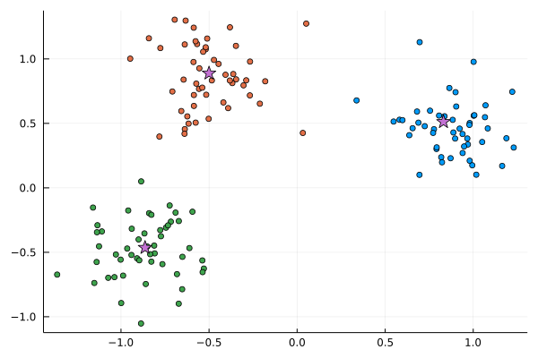
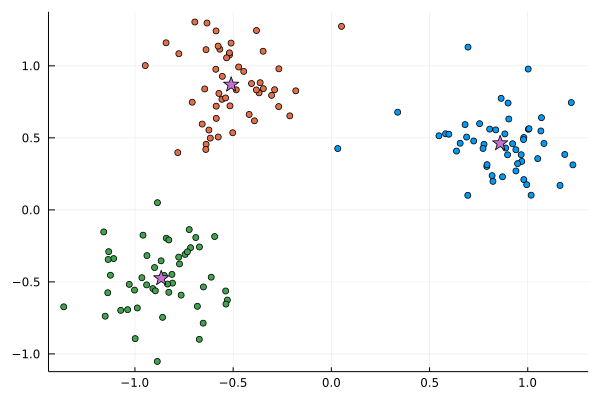
The centers of the clusters are
C_means = vcat([mean(X[L .== i,:], dims=1) for i in 1:k]...)
3×2 Matrix{Float64}:
  0.859565   0.461871
 -0.510111   0.869056
 -0.866179  -0.474655
scatter(X[:,1], X[:,2], c=L; leg=:none)
scatter!(C_means[:,1], C_means[:,2], c=4, markershape=:star, ms=8)
Now, we use define clustering as the SGD optimization problems.
Given $n$ observations ${x_1,\ldots,x_n}$, the observations are assigned to $k$ clusters $K={C_1,\ldots,C_k}$ so as to minimize a distance between points and the centers of the clusters,
$$\arg\min_K \sum_{C_i \in K} \sum_{x \in C_i} ||x - \mu_i||^2$$
where $\mu_i$ is a mean of the cluster $C_i$.
The above problem is a combinatorial optimization interpretation of the $k$-means clustering.
We need to rewrite it to make useful in the SGD optimization setup.
We define a set of parameters $\boldsymbol{w} = {\mu_1, \ldots, \mu_k}$, and use these weights to optimize a model function $f_\boldsymbol{w}: \mathbb{R}^n \to \mathbb{R}$ that minimizes distance between dataset points $x_i \in \mathbb{R}^n$ and the corresponding cluster centers $\mu_i \in \mathbb{R}^n$,
$$ f_\boldsymbol{w}(x) = || x - \mu_* ||{\mu* \in \boldsymbol{w}}^2 $$
where the $\mu_*$ is the closest of the current means from the weights vector $\boldsymbol{w}$ to the given point $x$,
$$|| x - \mu_* ||^2 \leq || x - \mu_i ||^2, ; 1\leq i \leq k$$
Now, the combinatorial optimization problem can be reshaped into the following minimization problem,
$$\arg\min_\boldsymbol{w} \sum_{x} f_\boldsymbol{w}(x)$$
We’ve hidden the combinatorial part of the problem in the model function. The the closed-form gradient expression is hardly possible, but we’ll estimate the gradient numerically though the automatic differentiation.
Instead of storing the clusters centers as a collection of the separate $\mathbb{R}^n$ vectors, we keep them in the stacked matrix form, so the parameter vector defined as $\boldsymbol{w} \in \mathbb{R}^{k \times n}$.
First, we define our model function. The cluster centers are decoded from the weight vector, and the minimal distance to the particular cluster center is reported.
# find minimum distance to each mean
nearest(w, x) = findmin([norm(vec(x) - μ)^2 for μ in eachrow(w)])
nearest (generic function with 1 method)
assignments(w, x) = nearest(w, x) |> last
cl_model(w, x) = nearest(w, x) |> first
cl_model (generic function with 1 method)
Next, we run SGD with randomly initialize cluster center parameters. We pass the original dataset without any additional labeling information.
- The clustering problem is an unsupervised leaning technique. It only requires the original data without any information on the original points’ class assignments. Our model function performs estimation of the parameters weights based on the global properties of the dataset, rather then by comparison to the original class assignments.
- The batch size is set to
1, so we won’t conflate loss from points in various cluster in the gradient estimation.
Random.seed!(42)
w = randn(k,size(X,2))
println("μs: $w")
sgd!(w, cl_model, X, η=0.05, ε=1e-6, maxiter=5000, skip=500, batch=1)
μs: [-0.5560268761463861 -0.29948409035891055; -0.444383357109696 1.7778610980573246; 0.027155338009193845 -1.14490153172882]
Itr: 500, w=[0.82731 0.57668; -0.48511 0.92632; -0.91179 -0.48728], ∇w=[-0.01791 0.0087; 0.0 0.0; 0.0 0.0], |∇w|=0.019911866852457844
Itr: 1000, w=[0.8749 0.50064; -0.53769 0.81063; -0.88703 -0.46346], ∇w=[0.0 0.0; 0.0 0.0; 0.01325 0.00501], |∇w|=0.014162135339204412
Itr: 1500, w=[0.84462 0.54373; -0.52102 0.85063; -0.84259 -0.49378], ∇w=[0.11158 0.01108; 0.0 0.0; 0.0 0.0], |∇w|=0.11213199077301116
Itr: 2000, w=[0.83976 0.56397; -0.56008 0.82763; -0.87795 -0.53167], ∇w=[0.6412 -0.14564; 0.0 0.0; 0.0 0.0], |∇w|=0.6575297941582268
Itr: 2500, w=[0.84617 0.48442; -0.4848 0.86746; -0.83688 -0.48416], ∇w=[0.0 0.0; 0.0 0.0; -0.00016 0.00013], |∇w|=0.00020590556058078827
Itr: 3000, w=[0.89167 0.51402; -0.52747 0.81136; -0.83358 -0.49429], ∇w=[-0.0 -0.0; -0.0 -0.0; -0.05609 -0.08199], |∇w|=0.09933852558088195
Itr: 3500, w=[0.86444 0.55479; -0.43645 0.87238; -0.89263 -0.46444], ∇w=[0.0 0.0; 0.00805 0.00752; 0.0 0.0], |∇w|=0.01101637671251697
Converged after 3661 iterations

3×2 Matrix{Float64}:
  0.854279   0.503016
 -0.382621   0.830109
 -0.895628  -0.517351
Now, we can compute assignments of the points to the found cluster centers.
C = [assignments(w, x) for x in eachrow(X)]
scatter(X[:,1], X[:,2], c=C; leg=:none)
scatter!(w[:,1], w[:,2], c=4, markershape=:star, ms=8)

Original cluster centers
C_means
3×2 Matrix{Float64}:
  0.859565   0.461871
 -0.510111   0.869056
 -0.866179  -0.474655
SGD estimated cluster centers
reshape(w, k, 2)[[1,2,3],:]
3×2 Matrix{Float64}:
  0.854279   0.503016
 -0.382621   0.830109
 -0.895628  -0.517351
abs(norm(C_means) - norm(w))
0.01613823457164032
Flux.jl
Flux.jl is a powerful ML package which provides abstractions for ML algorithms/workflow. We use package’s optimization functionality for solving our clustering problem.
We use ADAM optimizer, one of the advanced SGD optimizer in our optimization setup.
using Flux
α = 0.01
opt = ADAM(α)
ADAM(0.01, (0.9, 0.999), IdDict{Any, Any}())
We generate randomly centers of the clusters.
Random.seed!(42)
μs = randn(k,size(X,2))
p = params(μs)
μs
3×2 Matrix{Float64}:
 -0.556027   -0.299484
 -0.444383    1.77786
  0.0271553  -1.1449
Define a loss functions as a square of the distance to the closest cluster center.
loss(x) = cl_model(μs, x).^2
loss (generic function with 2 methods)
Now, we run optimization algorithm for several iterations to find optimal cluster centers.
for i in 1:15
    Flux.train!(loss, p, eachrow(X), opt)
    println("$i: loss = $(sum(loss,eachrow(X)))")
end
μs
1: loss = 93.13811449403909
2: loss = 31.164874794255102
3: loss = 12.206903589253189
4: loss = 6.43721086580895
5: loss = 4.38488807194685
6: loss = 3.4809445023868384
7: loss = 3.0315340369883255
8: loss = 2.7912553240566274
9: loss = 2.658689795036094
10: loss = 2.5856409003074488
11: loss = 2.534053082042835
12: loss = 2.4447487135885204
13: loss = 2.3997128064432163
14: loss = 2.376734171151653
15: loss = 2.3663889456009857

3×2 Matrix{Float64}:
  0.83104    0.511826
 -0.500088   0.888695
 -0.863375  -0.464023
The found solution is very close to the true cluster centers.
C_means
3×2 Matrix{Float64}:
  0.859565   0.461871
 -0.510111   0.869056
 -0.866179  -0.474655
abs(norm(C_means) - norm(μs))
0.0029069619012374037
C = [assignments(μs, x) for x in eachrow(X)]
scatter(X[:,1], X[:,2], c=C; leg=:none)
scatter!(μs[:,1], μs[:,2], c=4, markershape=:star, ms=8)