Discrete Random Variables and Their Distributions
Random Variables
A variable whose value is based on the outcome of a random event is called a random variable.
If we can list all possible outcomes, the random variable is called a discrete random variable.
If a random variable can take on any value between two values, it is called a continuous random variable.
Example 1
Consider an experiment of tossing 3 fair coins and counting the number of heads.
Let $X$ be the number of heads. Prior to an experiment, its value is not known. All we can say is that $X$ has to be an integer between 0 and 3. Since assuming each value is an event, we can compute probabilities,
Discrete Distribution
Collection of all the probabilities related to $X$ is the distribution of X. The function $P(x) = P\{X=x\}$ is the probability mass function, or pmf.
The cumulative distribution function, or cdf is defined as $F(x) = P\{X \leq x\} = \sum_{y\leq x}P(y)$
The set of possible values of $X$ is called the support of the distribution $F$.
Distribution probabilities
For any set $A$,
When $A$ is an interval, its probability can be computed directly from the cdf $F(x)$, $P \{a < X \leq b\} = F(b) - F(a)$
Example 2
A program consists of two modules. The number of errors $X_1$ in the first module has the pmf $P_1(x)$, and the number of errors $X_2$ in the second module has the pmf $P_2(x)$, independently of $X_1$, if
| x | $P_1(x)$ | $P_2(x)$ |
|---|---|---|
| 0 | 0.5 | 0.7 |
| 1 | 0.3 | 0.2 |
| 2 | 0.1 | 0.1 |
| 3 | 0.1 | 0.0 |
Find the pmf and cdf of $Y = X_1 + X_2$, the total number of errors.
Joint and marginal distributions
If $X$ and Y are random variables, then the pair $(X, Y)$ is a random vector.
Its distribution is called the joint distribution of $X$ and $Y$.
Individual distributions of $X$ and $Y$ are then called the marginal distributions.
Joint probability distribution
Joint probability mass function of $X$ and $Y$ is
If ${(X, Y ) = (x, y)}$ are exhaustive and mutually exclusive events for different pairs $(x, y)$, therefore,
Addition Rule
Addition Rule: computing marginal probabilities from the joint distribution.
Independence
Random variables $X$ and $Y$ are independent if
for all values of $x$ and $y$.
This means, events $\{X = x\}$ and $\{Y = y\}$ are independent for all $x$ and $y$.
Example 3
A program consists of two modules. The number of errors, $X$, in the first module and the number of errors, $Y$, in the second module have the joint distribution, $P(0, 0) = P(0, 1) = P(1, 0) = 0.2$, $P(1, 1) = P(1, 2) = P(1, 3) = 0.1$, $P(0, 2) = P(0, 3) = 0.05$. Find:
the marginal distributions of $X$ and $Y$
the probability of no errors in the first module
the distribution of the total number of errors in the program
find out if errors in the two modules occur independently.
Expectation and Variance
Expectation or expected value of a random variable $X$ is its mean, the average value. It's denoted by $E[X]$, and defined by
Expected value is often denoted by a Greek letter $\mu$.
Expectation of a function: $E[g(X)] = \sum_x g(x) P(X=x)$
Properties of Expectations
For any random variables $X$ and $Y$ and any non-random numbers $a$ and $c$ $E(X + Y) = E(X) + E(Y)$ $E(aX) = a E(X)$ $E(c) = c$
For independent $X$ and $Y$, $E(XY) = E(X)E(Y)$
Example 4
What are the expected values of $X$, $Y$, and $X+Y$ from Ex. 3?
Variance
Variance of a random variable is defined as the expected squared deviation from the mean. For discrete random variables, variance is
or
it equals 0 only if $x = \mu$ for all values of $x$, i.e., when $X$ is constantly equal to $\mu$.
a constant (non-random) variable has zero variability.
Standard Deviation
Standard deviation is a square root of variance $\sigma = Std(X) = \sqrt{Var(X)}$
Covariance
Covariance is the expected product of deviations of $X$ and $Y$ from their respective expectations, which summarizes interrelation of two random variables.
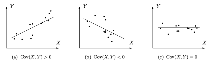
Covariance $\sigma_{XY} = Cov(X,Y)$ is defined as
Correlation
If $Cov(X,Y)=0$, we say that $X$ and $Y$ are uncorrelated.
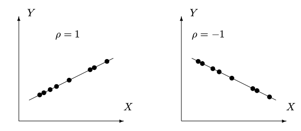
Correlation coefficient between variables $X$ and $Y$ is defined as
Correlation coefficient is a rescaled, normalized covariance.
Properties of Variances and Covariances
For independent $X$ and $Y$,
Example 5
What are the variance, std. deviation, covariance, and correlation values of $X$, $Y$, and $X+Y$ from Ex. 3?
Chebyshev's Inequality
Any random variable $X$ with expectation $\mu = E(X)$ and variance $\sigma^2 = Var(X)$ belongs to the interval $\mu \pm \varepsilon$ with probability of at least $1-(\sigma/\varepsilon)^2$ . That is
for any distribution with expectation $\mu$ and variance $\sigma^2$ and for any positive $\varepsilon$.
Example 6
Suppose the number of errors in a new software has expectation $\mu = 20$ and a standard deviation of 2.
What is the probability that there more than 30 errors?
What is the probability that there more than 30 errors for a standard deviation of 5?
Discrete Distributions
Bernoulli Distribution
A random variable with two possible values, 0 and 1, is called a Bernoulli variable, its distribution is Bernoulli distribution, and any experiment with a binary outcome is called a Bernoulli trial.
If $P(1) = p$ is the probability of a success,
then $P(0) = q = 1 - p$ is the probability of a failure.
Binomial Distribution
A variable described as the number of successes in a sequence of independent Bernoulli trials has Binomial distribution. Its parameters are $n$, the number of trials, and $p$, the probability of success.
Binomial Distribution: Expectation and Variance
Any Binomial variable $X$ can be represented as a sum of independent Bernoulli variables,
Thus, Binomial expectation and variance can be calculated as follows
Example 7
An exciting computer game is released. Sixty percent of players complete all the levels. Thirty percent of them will then buy an advanced version of the game. Among 15 users, what is the expected number of people who will buy the advanced version?
What is the probability that at least two people will buy it?
Example 8
Consider the situation of a multiple-choice exam. It consists of 10 questions, and each question has four alternatives (of which only one is correct).
Calculate the probability that you answered the first question correctly and the second one incorrectly.
You will pass the exam if you answer six or more questions correctly. What is the probability that you will pass?
Geometric Distribution
The number of Bernoulli trials needed to get the first success has Geometric distribution.
for $x=1,2, \ldots$
Example 9
A driver looking for at a parking space down the street. There are five cars in front of the driver, each of which having a probability 0.2 of taking the space.
What is the probability that the car immediately ahead will enter the parking space?
Poisson Distribution
The number of rare events occurring within a fixed period of time has Poisson distribution.
Let $\lambda$ is a frequency (or average number) of events, then
Example 10
Customers of an internet service provider initiate new accounts at the average rate of 10 accounts per day.
What is the probability that more than 8 new accounts will be initiated today?
What is the probability that more than 16 accounts will be initiated within 2 days?
Poisson Approximation of Binomial Distribution
Poisson distribution can be effectively used to approximate Binomial probabilities when the number of trials $n$ is large, and the probability of success $p$ is small.
Example 11
Ninety-seven percent of electronic messages are transmitted with no error.
What is the probability that out of 200 messages, at least 195 will be transmitted correctly?