Hypothesis Testing
Example 1
Is the Dow Jones just as likely to move higher as it is to move lower on any given day?
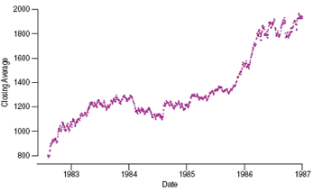
Out of the 1112 trading days in that period, the average increased on 573 days (sample proportion = 0.5153 or 51.53%).
It far enough from 50% to cast doubt on the assumption of equally likely up or down movement?
To test whether the daily fluctuations are equally likely to be up as down, we assume that they are, and that any apparent difference from 50% is just random fluctuation.
Hypotheses
The null hypothesis, $H_0$, specifies a population model parameter and proposes a value for that parameter.
We usually write a null hypothesis about a proportion in the form $H_0: p = p_0$.
For our hypothesis about the DJIA, we need to test $H_0: p = 0.5$.
The alternative hypothesis, $H_A$, contains the values of the parameter that we consider plausible if we reject the null hypothesis.
Our alternative is $H_A: p \neq 0.5$.
Alternative Hypotheses
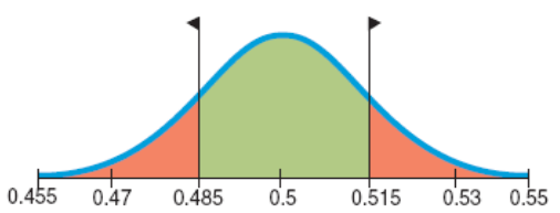
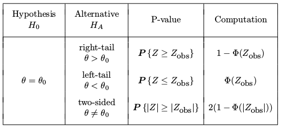
In a two-sided alternative we are equally interested in deviations on either side of the null hypothesis value
the P-value is the probability of deviating in either direction from the null hypothesis value.
An alternative hypothesis that focuses on deviations from the null hypothesis value in only one direction is called a one-sided alternative.
P-Values
The P-value is the probability of seeing the observed data (or something even less likely) given the null hypothesis.
A low enough P-value says that the data we have observed would be very unlikely if our null hypothesis were true.
If you believe in data more than in assumptions, then when you see a low P-value you should reject the null hypothesis.
When the P-value is high (or just not low enough), data are consistent with the model from the null hypothesis, and we have no reason to reject the null hypothesis.
Example 2
Which of the following are true?
A very low P-value provides evidence against the null hypothesis.
A high P-value is strong evidence in favor of the null hypothesis.
A P-value above 0.10 shows that the null hypothesis is true.
If the null hypothesis is true, you can't get a P-value below 0.01.
Example 2 (cont.)
Which of the following are true?
A very low P-value provides evidence against the null hypothesis.
True
A high P-value is strong evidence in favor of the null hypothesis.
False. A high p-value says the data are consistent with the null hypothesis.
A P-value above 0.10 shows that the null hypothesis is true.
False. No p-value ever shows that the null hypothesis is true (or false).
If the null hypothesis is true, you can't get a P-value below 0.01.
False. This will happen 1 in 100 times.
Alpha Levels and Significance
We can define a "rare event" arbitrarily by setting a threshold for our P-value, alpha level, $\alpha$.
If the P -value $< \alpha$ then reject $H_0$.
If the P -value $\geq \alpha$ then fail to reject $H_0$.
We call such results statistically significant.
Example 1 (cont.)
Find the standard deviation of the sample proportion of days on which the DJIA increased.
We've seen 51.53% up days out of 1112 trading days.
The sample size of 1112 is big enough to satisfy the Success/Failure condition.
We suspect that the daily price changes are random and independent.
Example 1 (cont.)
If we assume that the DJIA increases or decreases with equal likelihood, we'll need to center our Normal sampling model at a mean of 0.5.
Then, the standard deviation of the sampling
Example 1 (cont.)
How likely is it that the observed value would be 0.5153 - 0.5 = 0.0153 units away from the mean?
The exact probability is about 0.308. (Calculate.)
This is the probability of observing more than 51.53% up days (or more than 51.53% down days) if the null model were true.
That's not unusual, so there's really no convincing evidence that the market did not act randomly.
The Reasoning of Hypothesis Testing
Four sections: hypothesis, model, mechanics, and conclusion.
Hypotheses
First, state the null hypothesis, $H_0$: parameter = hypothesized value.
The alternative hypothesis, $H_A$, contains the values of the parameter we consider plausible when we reject the null.
Testing hypothesis is based on a test statistic $T$, a quantity computed from the data that has some known.
The Reasoning of Hypothesis Testing (cont.)
Model
Specify the model for the sampling distribution of the statistic you will use to test the null hypothesis and the parameter of interest. For proportions, use the Normal model for the sampling distribution.
State assumptions and check any corresponding conditions. For a test of a proportion, the assumptions and conditions are the same as for a one-proportion z-interval.
The Reasoning of Hypothesis Testing (cont.)
Your model step should end with a statement such as:
Because the conditions are satisfied, we can model the sampling distribution of the proportion with a Normal model.
Each test has a name that you should include in your report. The test about proportions is called a one-proportion z-test.
One-proportion Z-test
The conditions for the one-proportion z-test are the same as for the one-proportion z-interval. We test the hypothesis $H_0:p=p_0$ using the statistic $z = \frac{\hat{p} - p_0}{SD(\hat{p})}$
We also use to find the standard deviation as $SD(\hat{p}) = \sqrt{p_0q_0/n}$
When the conditions are met and the null hypothesis is true, this statistic follows the standard Normal model, so we can use that model to obtain a P-value.
The Reasoning of Hypothesis Testing (cont.)
Mechanics
Perform the actual calculation of our test statistic from the data. Usually, the mechanics are handled by a statistics program or calculator.
The goal of the calculation is to obtain a P-value.
If the P-value is small enough, we'll reject the null hypothesis.
The Reasoning of Hypothesis Testing (cont.)
Conclusions and Decisions
The primary conclusion in a formal hypothesis test is only a statement stating whether we reject or fail to reject that hypothesis.
Your conclusion about the null hypothesis should never be the end of the process. You can't make a decision based solely on a P-value.
Example 3
A survey of 100 CEOs finds that 60 think the economy will improve next year. Is there evidence that the rate is higher among all CEOs than the 55% reported by the public at large?
Find the standard deviation of the sample proportion based on the null hypothesis.
Find the z-statistic.
Does the z-statistic seem like a particularly large or small value?
Example 3 (cont.)
A survey of 100 CEOs finds that 60 think the economy will improve next year. Is there evidence that the rate is higher among all CEOs than the 55% reported by the public at large?
Find the standard deviation of the sample proportion based on the null hypothesis.
$SE(\hat{p}) = \sqrt{p_0q_0/n} = 0.0497$
Find the z-statistic.
$z = (\hat{p} - p) / SE(\hat{p}) = 1.006$
Does the z-statistic seem like a particularly large or small value?
No, this is not an unusual value for z.
Two Types of Errors
We can make mistakes in two ways:
(False Hypothesis) The null hypothesis is true, but we mistakenly reject it.
(False Negative) The null hypothesis is false, but we fail to reject it.
These two types of errors are known as Type I and Type II errors respectively.
Two Types of Errors (cont.)
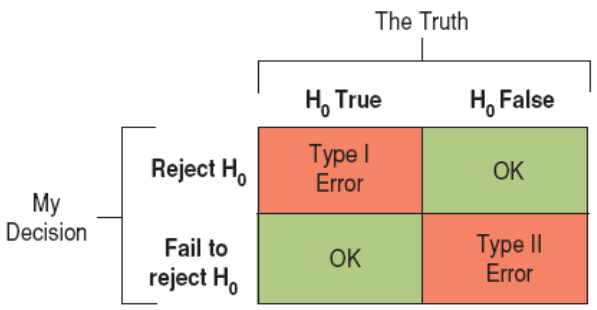
When you choose level $\alpha$, you're setting the probability of a Type I error to $\alpha$.
Significance Level & Power
Probability of a type I error is the significance level of a test,
A test's ability to detect a false hypothesis is called the power of the test.
The power of a test is the probability that it correctly rejects a false null hypothesis.
We know that $\beta$ is the probability that a test fails to reject a false null hypothesis, so the power of the test is the complement, $1 - \beta$.
Critical Values
A critical value, $z^\ast$, corresponds to a selected confidence level.
Here are the traditional $z^\ast$ critical values from the Normal model:
| $\alpha$ | 1-sided | 2-sided |
|---|---|---|
| 0.05 | 1.645 | 1.96 |
| 0.01 | 2.33 | 2.576 |
| 0.001 | 3.09 | 3.29 |
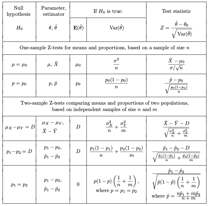
P-values for Z-tests
One-Sample T-Test
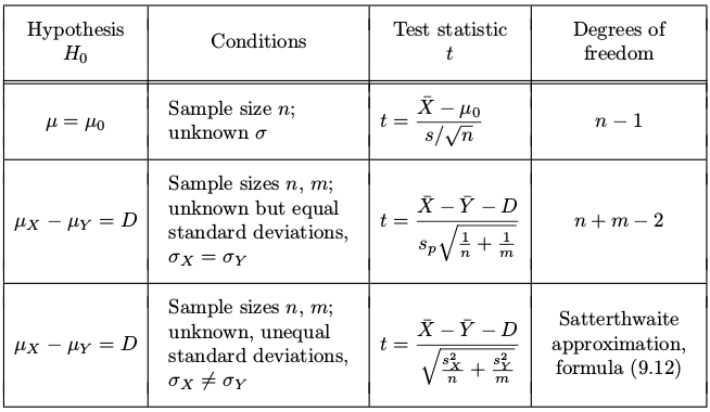
For testing a hypothesis about a mean, the test is based on the Student's T-distribution.
Is there evidence from a sample that the mean is really different from some hypothesized value calls for a one-sample t-test for the mean.
One-sample T-test for the mean
The conditions for the one-sample t-test for the mean are the same as for the one-sample t-interval. We test the hypothesis $H_0: \mu = \mu_0$ using the statistic
where the standard error of is $SE(\bar{y}) = s/\sqrt n$
When the conditions are met and the null hypothesis is true, this statistic follows a Student's t-model with degrees of freedom. We use that model to obtain a P-value.
Example 4
A new manager of a small convenience store randomly samples 20 purchases from yesterday's sales. If the mean was 45.26 and the standard deviation was 20.67, is there evidence that the mean purchase amount is at least 40?
What is the null hypothesis?
Find the t-statistic.
What is the P-value of the test statistic?
What do you tell the store manager about the mean sales?
Example 4 (cont.)
What is the null hypothesis?
Find the t-statistic.
What is the P-value of the test statistic?
What do you tell the store manager about the mean sales?
Fail to reject the null hypothesis. There is insufficient evidence that the mean sales is greater than 40.
Confidence Intervals and Hypothesis Tests
Because confidence intervals are naturally two-sided, they correspond to two-sided tests.
In general, a confidence interval with a confidence level of C% corresponds to a two-sided hypothesis test with an $\alpha$ level of 100 - C%.
A one-sided confidence interval leaves one side unbounded.
A one-sided confidence interval can be constructed from one side of the associated two-sided confidence interval.
Example 5
Recall the new manager of a small convenience store who randomly sampled 20 purchases from yesterday's sales.
Given a 95% confidence interval (35.586, 54.934), is there evidence that the mean purchase amount is different from 40?
Is the confidence interval conclusion consistent with the (two-sided) P-value = 0.2692?
Example 5 (cont.)
Given a 95% confidence interval (35.586, 54.934), is there evidence that the mean purchase amount is different from 40?
At $\alpha = 0.05$, fail to reject the null hypothesis. The 95% confidence interval contains 40 as a plausible value.
Is the confidence interval conclusion consistent with the (two-sided) P-value = 0.2692?
Yes, the hypothesis test conclusion is consistent with the confidence interval.
Comparing Two Means
The statistic of interest is the difference in the observed means of the offer and no offer groups: $y_0 - y_n$.
What we'd really like to know is the difference of the means in the population at large: $\mu_0 - \mu_n$.
Now the population model parameter of interest is the difference between the means.
Comparing Two Means (cont.)
As long as the two groups are independent, we find the standard deviation of the difference between the two sample means by adding their variances and then taking the square root:
Comparing Two Means (cont.)
Usually we don't know the true standard deviations of the two groups, $\sigma_1$ and $\sigma_2$, so we substitute the estimates, $s_1$ and $s_2$, and find a standard error:
We'll use the standard error to see how big the difference really is.
A Sampling Distribution for the Difference Between Two Means
When the conditions are met, the standardized sample difference between the means of two independent groups,
can be modeled by a Student's $t$-model with a number of degrees found with a special formula.
Rough approximation: df $= n_1 + n_2 - 2$
Satterthwaite approximation:
The Two-Sample T-Test
Test hypothesis:
where the hypothesized difference $\Delta_0$ is almost always 0.
When the null hypothesis is true, the statistic can be closely modeled by a Student's t-model with a number of degrees of freedom given by a special formula.
Assumptions and Conditions
Independence Assumption: The data in each group must be drawn independently and at random.
Randomization Condition: Without randomization of some sort, there are no sampling distribution models and no inference.
10% Condition: We usually don't check this condition for differences of means. We need not worry about it at all for randomized experiments.
Normal Population Assumption: underlying populations are each Normally distributed.
Nearly Normal Condition: We must check this for both groups; a violation by either one violates the condition.
Independent Groups Assumption: the two groups we are comparing must be independent of each other.
CI for the Difference Between Two Means
When the conditions are met, we are ready to find a two-sample $t$-interval for the difference between means of two independent groups, $\mu_1 - \mu_2$. The confidence interval is:
Example 6
A market analyst wants to know if a new website is showing increased page views per visit. Given statistics below, find the estimated mean difference in page visits between the two websites.
| Website 1 | Website 2 |
|---|---|
| $n_1 = 80$ | $n_1 = 95$ |
| $\hat{y}_1 = 7.7$ pages | $\hat{y}_2 = 7.3$ pages |
| $s_1 = 4.6$ pages | $s_1 = 4.3$ pages |
Example 6 (cont.)
where df = 163.59
Fail to reject the null hypothesis. Since 0 is in the interval, it is a plausible value for the true difference in means.
Example 6 (cont.)
where df = 163.59
Fail to reject the null hypothesis. There is insufficient evidence to conclude a statistically significant mean difference in the number of webpage visits.
The Pooled T-Test
If we assume that the variances of the groups are equal (at least when the null hypothesis is true), then we can save some degrees of freedom.
To do that, we have to pool the two variances that we estimate from the groups into one common, or pooled, estimate of the variance:
The Pooled T-Test (cont.)
Now we substitute the common pooled variance for each of the two variances in the standard error formula, making the pooled standard error formula simpler:
The formula for degrees of freedom for the Student's $t$-model is simpler, too.
The Pooled T-Test
For pooled $t$-methods, the Equal Variance Assumption need to be satisfied that the variances of the two populations from which the samples have been drawn are equal. That is, $\sigma_1 = \sigma_2$.
where the hypothesized difference $\Delta_0$ is almost always 0, using the statistic
The Pooled T-Test Confidence Interval
The corresponding pooled-$t$ confidence interval is
where the critical value $t^*$ depends on the confidence level and is found with $(n_1-1) + (n_2-1)$ degrees of freedom.
Summary of T-tests
Inference about Variances
We need special treatment for confidence intervals and tests for the variance, because
variance is a scale and not a location parameter,
the distribution of its estimator, the sample variance, is not symmetric.
Chi-square Distribution
When observations $X_1, \ldots, X_n$ are independent and Normal with $Var(X_i) = \sigma^2$, the distribution of
is Chi-square with $(n-1)$ degrees of freedom.
Chi-square distribution, or $\chi^2$, is a continuous distribution with density
or Chi-square($\nu$) = Gamma($\nu$/2, 1/2) with E(X)=$\nu$ and Var(X)=$2\nu$.
Chi-square Densities
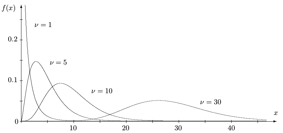
Chi-square densities with $\nu$ = 1, 5, 10, and 30 degrees of freedom. Each distribution is right-skewed. For large $\nu$, it is approximately Normal.
CI for the Population Variance
Let us construct a $(1-\alpha)100\%$ confidence interval for the population variance $\sigma^2$, based on a sample of size $n$.
Then confidence interval for the variance is
Example 7
A sample from the measurement device of 6 measurements:
2.5, 7.4, 8.0, 4.5, 7.4, 9.2with the known standard deviation $\sigma$ = 2.2. Using the data only, construct a 90% confidence interval for the standard deviation.
Example 7 (cont.)
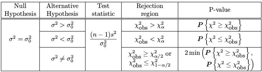
Testing Variance
Testing the population variance with $\chi^2$-tests
Example 8
Refer to example 7. The 90% confidence interval constructed there contains the suggested value of $\sigma$ = 2.2. Then, by duality between confidence intervals and tests, there should be no evidence against this value of $\sigma$. Measure the amount of evidence against it by computing the suitable P-value.
Example 8 (cont.)
The hypothesis $H_0: \sigma = 2.2$ is tested against $H_A: \sigma \neq 2.2$.
Compute the test statistic from the data
with $\nu = n - 1 = 5$ degrees of freedom,
Therefore,
The evidence against $\sigma = 2.2$ is very weak; at all typical significance levels $H_0$ should be accepted.