Statistics
Variable Types
Categorical or qualitative
when a variable names categories and answers questions about how cases fall into those categories
Quantitative
when a variable has measured numerical values with units and the variable tells us about the quantity of what is measured
Example 1
Size (acres) [quantitative]
Number of years in existence [quantitative]
State [categorical] [an indicator variable]
Varieties of grapes grown [categorical]
Average case price [quantitative]
Gross sales [quantitative]
Percent profit [quantitative]
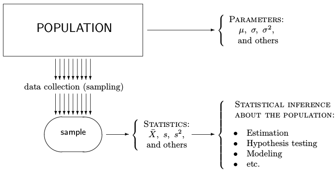
Population and Sample
A population consists of all units of interest. Any numerical characteristic of a population is a parameter, $\theta$.
A sample consists of observed units collected from the population. It is used to make statements about the population. Any function of a sample is called statistic.
In order to know the population parameters, one must measure the entire population, i.e., to conduct a census.
Parameters
Parameters can be estimated a form of a random population sample up to a certain measurable degree of accuracy.
Errors
Sampling errors are caused by the mere fact that only a sample, a portion of a population, is observed.
For most of reasonable statistical procedures, sampling errors decrease as the sample size increases.
Non-sampling errors are caused by inappropriate sampling schemes or wrong statistical techniques.
Often no wise statistical techniques can rescue a poorly collected sample of data.
Sampling Designs
Simple Random Sample (SRS)
A sample drawn so that every possible sample has an equal chance of being selected is called a simple random sample.
With this method each combination of individuals has an equal chance of being selected as well.
A sampling frame is a list of individuals from which the sample will be drawn.
A sample-to-sample differences in values of measured variables is sampling variability.
Stratified Sampling
The population is sliced into homogeneous groups, strata
Use SRS within each stratum
Combine the results at the end
Reduced sampling variability is the most important benefit of stratifying.
Cluster and Multistage Sampling
Clustering sampling
Splitting the population into parts or clusters that each represent the population
Performing a census within one or a few clusters at random is called cluster sampling.
If each cluster fairly represents the population, cluster sampling will generate an unbiased sample.
Multistage samples
Sampling schemes that combine several methods
Systematic Samples
A systematic sample is created by selecting systematically.
For example, we might select every tenth person on an alphabetical list of employees.
To make sure our sample is random, we still must start the systematic selection with a randomly selected individual.
Example 2
Researchers waited outside a bar they had randomly selected from a list of such establishments. They stopped every 10th person who came out of the bar and asked whether he or she thought drinking and driving was a serious problem. Identify the population of interest, population parameter, sampling frame and method.
Population of interest
Population parameter
Sampling frame
Method
Example 2 (cont.)
Population of interest: U.S. adults
Population parameter: Proportion who think drinking and driving is a serious problem
Sampling frame: Bar patrons
Method: Systematic sampling
Example 3
An amusement park has opened a new roller coaster. It is so popular that people are waiting for up to 3 hours for a 2-minute ride. Concerned about how patrons feel about this, they survey every 10th person on the line for the roller coaster, starting from a randomly selected individual. Identify sampling frame. Is the sample likely to be representative?
Sampling frame
Representative
Example 3 (cont.)
Sampling frame: Patrons in line on that day at that time.
Representative: No. Only those who think it worth the wait are likely to be in line. Also, those who don't like roller coasters aren't in the sampling frame, so the poll will not get a fair picture of whether park patrons feel about long lines for roller coaster rides.
Bad Sampling
Voluntary Response Sample
A large group of individuals is invited to respond, and all who do respond are counted
Voluntary response samples are almost always biased
Often biased toward those with strong opinions or those who are strongly motivated
Often hard to define the sampling frame
Convenience Sampling
In convenience sampling we simply include the individuals who are convenient.
This group may not be representative of the population.
Bad Sampling Frame
An SRS from an incomplete sampling frame introduces bias because the individuals included may differ from the ones not in the frame.
Undercoverage
Some portion of the population is not sampled at all or has a smaller representation in the sample than it has in the population.
Rather than sending out a large number of surveys for which the response rate will be low, it is often better to design a smaller, randomized survey for which you have the resources to ensure a high response rate.
Example 4
We want to know what percentage of local doctors accept Medicaid patients. We call the offices of 50 doctors randomly selected from local Yellow Pages listings. Is this sampling method appropriate? If not, identify the problem.
Is this method appropriate?
Example 4 (cont.)
We want to know what percentage of local doctors accept Medicaid patients. We call the offices of 50 doctors randomly selected from local Yellow Pages listings. Is this sampling method appropriate? If not, identify the problem.
Method appropriate: Depends on the Yellow Page listing used. If from regular listings, this is fair if all doctors are listed. If from ads, then probably not as those doctors may not be typical.
Simple Descriptive Statistics
Shape
When you describe a distribution, you should pay attention to its:
shape
center
spread
We describe the shape of a distribution in terms of its modes, its symmetry, and whether it has any gaps or outlying values.
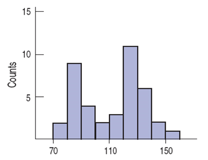
Mode
Peaks or humps seen in a histogram are called the modes of a distribution.
A distribution whose histogram has
one main peak is called unimodal
two peaks - bimodal
three or more - multimodal
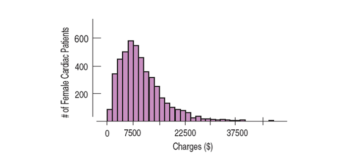
Symmetry
A distribution is symmetric if the halves on either side of the center look, at least approximately, like mirror images.
The thinner ends of a distribution are called the tails. If one tail stretches out farther than the other, the distribution is said to be skewed to the side of the longer tail.
Outliers
The outliers in a distribution are those values that stand off away from the body of the distribution.
can affect every statistical method we will study
can be the most informative part of your data
may be an error in the data
should be discussed in any conclusions drawn about the data
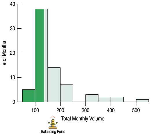
Mean
The mean of a distribution is calculated as sum of all values, $X_i$, and divided by the number of values, $N$.
The mean is considered to be the balancing point of the distribution.
Bias
An estimator $\hat{\theta}$ is unbiased for a parameter $\theta$ if its expectation equals the parameter, $E(\hat{\theta}) = \theta$ for all possible values of $\theta$.
Bias of $\hat{\theta}$ is defined as $Bias(\hat{\theta}) = E(\hat{\theta}) - \theta$
Consistency
An estimator $\hat{\theta}$ is consistent for a parameter $\theta$ if the probability of its sampling error of any magnitude converges to 0 as the sample size increases to infinity, $P\{ |\hat{\theta} - \theta| > \varepsilon \} \rightarrow 0, \; n \rightarrow \infty$
for any $\varepsilon > 0$.
That is, when we estimate $\theta$ from a large sample, the estimation error $|\hat{\theta} - \theta|$ is unlikely to exceed $\varepsilon$, and it does it with smaller and smaller probabilities as we increase the sample size, $n$.
Consistency follows directly from Chebyshev's inequality
Asymptotic Normality
By the Central Limit Theorem, the sum of observations, and therefore, the sample mean have approximately Normal distribution if they are computed from a large sample. That is, the distribution of
converges to Standard Normal as $n \rightarrow \infty$. This property is called Asymptotic Normality.
Median
The median is the value separating the higher half the data from lover part.
The median is resistant to unusual observations and to the shape of the distribution.
Spread
Sometimes we need to determine how spread out the data.
One simple measure of spread is the range, defined as the difference between the extremes.
The range is a single value and it is not resistant to unusual observations.
Quantile
A $p$-quantile of a population is such a number x that solves equations $ \begin{cases} P{X < x} \leq p \ P{X > x} \leq 1-p \end{cases} $
A sample $p$-quantile is any number that exceeds at most $100p$% of the sample, and is exceeded by at most $100(1 - p)$% of the sample.
A $\gamma$-percentile is $(0.01\gamma)$-quantile.
Quartiles
The quartiles of a ranked set of data values are the three points that divide the data set into four equal groups, each group comprising a quarter of the data.
The first quartile (Q1) is defined as the middle number between the smallest number and the median of the data set, 25th percentile
The second quartile (Q2) is the median of the data, 50th percentile
The third quartile (Q3) is the middle value between the median and the highest value of the data set, 75th percentile
Interquartile Range
The interquartile range (IQR) is defined to be the difference between the two quartile values.
Variance
For a sample $(X_1, \ldots, X_n)$, the average of the squared deviations of the values of the variable $X_i$ from the mean, $\bar{X}$, is called the sample variance and is denoted by $s^2$.
It measures variability among observations and estimates the population variance, $\sigma^2 = Var(X)$.
Taking the square root of the variance corrects this issue and gives us the standard deviation.
Standard error of an estimator $\hat{\theta}$ is its standard deviation, $\sigma(\hat{\theta}) = Std(\hat{\theta})$.
Guide
If the shape is skewed, the median and IQR should be reported.
If the shape is unimodal and symmetric, the mean and standard deviation and possibly the median and IQR should be reported.
If there are multiple modes, try to determine if the data can be split into separate groups.
If there are unusual observations point them out and report the mean and standard deviation with and without the values.
Always pair the median with the IQR and the mean with the standard deviation.
Graphical statistics
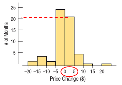
Histograms
A histogram is similar to a bar chart with the bin counts used as the heights of the bars. Note: there are no gaps between bars unless there are actual gaps in the data.
Boxplot
The five-number summary of a distribution reports its median, quartiles, and extremes (maximum and minimum).
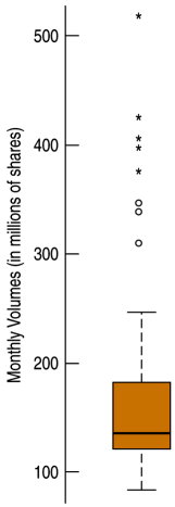
Boxplot (cont)
The central box shows the middle half of the data, between the quartiles – the height of the box equals the IQR.
If the median is roughly centered between the quartiles, then the middle half of the data is roughly symmetric.
If it is not centered, the distribution is skewed.The whiskers show skewness as well if they are not roughly the same length.
The outliers are displayed individually to keep them out of the way in judging skewness and to display them for special attention.
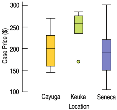
Example
Example: Wine Prices The boxplots displayed case prices (in dollars) of wines produces by vineyards along three of the Finger Lakes in upstate New York.
Which lake region produces the most expensive wine?
Which lake region produces the cheapest wine?
In which region are wines generally more expensive?
Example (cont.)
Seneca Lake
Seneca Lake
Keuka Lake
Cayuga Lake vineyards and Seneca Lake have approximately the same average case price of about 200, while a typical Keuka Lake vineyard has a case price of about 260. Keuka Lake vineyards have consistently high case prices, between 240 and 280, with one low outlier at about 170 per case. Cayuga Lake vineyards have case prices from 140 to 270, and Seneca Lake vineyards have highly variable case prices from 100 to 300.
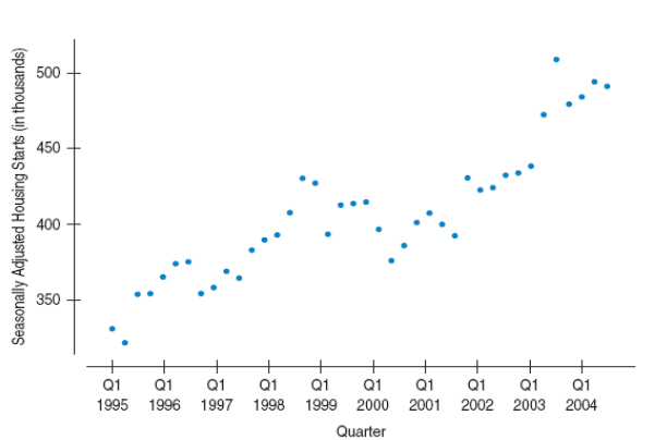
Scatterplot
Scatterplots are the ideal way to picture associations between two quantitative variables.
Other
A relative frequency histogram is displaying the percentage of cases in each bin instead of the count.
Stem-and-leaf displays are like histograms, but they also give the individual values.
Example: Create a stem-and-leaf display for the data 21, 22, 24, 33, 33, 36, 38, 41.
2|124
3|3368
4|1