Regression
Least Squares Estimation
Regression models relate a response variable to one or several predictors. Having observed predictors, we can forecast the response by computing its conditional expectation, given all the available predictors.
Response or dependent variable $Y$ is a variable of interest that we predict based on one or several predictors.
Predictors or independent variables $X^{(1)}, \ldots, X^{(k)}$ are used to predict the values and behavior of the response variable $Y$.
Regression of $Y$ on $X^{(i)}$ is the conditional expectation,
It is a function of $x^{(1)}, \ldots, x^{(k)}$ whose form can be estimated from data.
Method of Least Squares
In univariate regression, we observe pairs $(x _i, y_i)$.
For forecasting, we are looking for the function $G(x)$ that is close to the observed data points. This is achieved by minimizing distances between observed $y_i$ and the corresponding points on the fitted regression line, $\hat{y}_i = \hat{G}(x_i)$.
The difference between the predicted value $\hat{y}_i$ and the observed value, $y_i$, is called the residual and is denoted $e_i$.
Method of least squares finds a regression function $\hat{G}(x)$ that minimizes the sum of squared residuals
The Linear Model
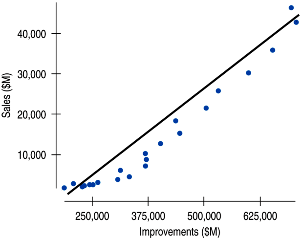
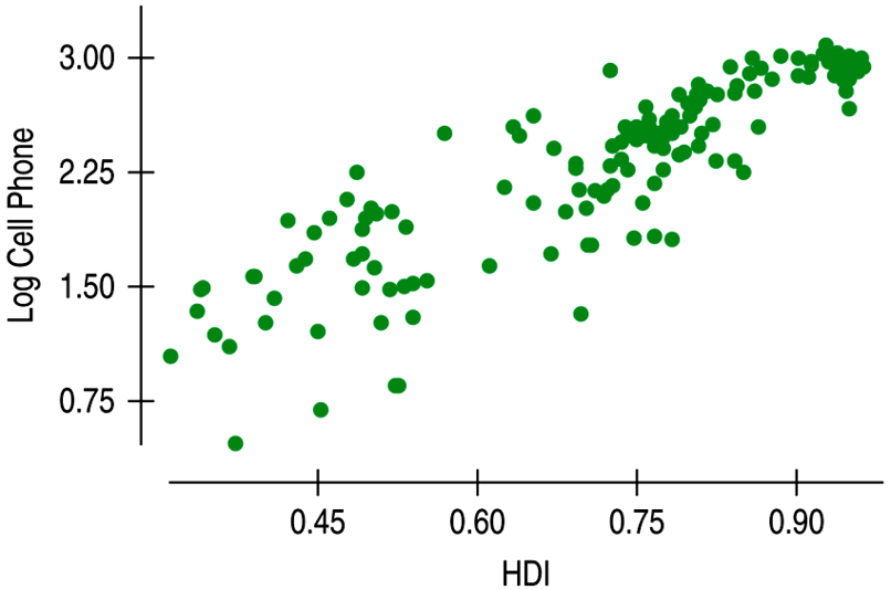
The scatterplot below shows Lowe's sales and home improvement expenditures between 1985 and 2007.
The relationship is strong, positive, and linear (r = 0.976).
The Linear Model (cont.)
We see that the points don't all line up, but that a straight line can summarize the general pattern. We call this line a linear model.
A linear model can be written in the form
where $\beta_0$ (slope) and $\beta_1$ (intersept) are numbers estimated from the data and $\hat{y}$ is the predicted value.
Example 1
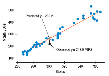
In the computer usage model for 301 stores, the model predicts 262.2 MIPS (Millions of Instructions Per Second) and the actual value is 218.9 MIPS. We may compute the residual for 301 stores.
Estimation in Linear Regression
Let us estimate the slope and intercept by method of least squares.
We minimize sum of sq. residuals by taking partial derivatives of $Q$, equating them to 0, and solving the equations for $\beta_0$ and $\beta_1$.
Estimation in Linear Regression (cont.)
From the first equation, $\beta_0 = \frac{\sum_i y_i - \beta_1 \sum_i x_i}{n} = \bar{y} - \beta_1 \bar{x}$
From the second equation,
where
Example 2
According to the International Data Base of the U.S. Census Bureau, population of the world grows according to below table. How can we use these data to predict the world population in years 2020 and 2030?
| Year | Population | Year | Population | Year | Population |
|---|---|---|---|---|---|
| 1950 | 2558 | 1975 | 4089 | 2000 | 6090 |
| 1955 | 2782 | 1980 | 4451 | 2005 | 6474 |
| 1960 | 3043 | 1985 | 4855 | 2010 | 6864 |
| 1965 | 3350 | 1990 | 5287 | 2020 | ? |
| 1970 | 3712 | 1995 | 5700 | 2030 | ? |
Regression and Correlation
We can find the slope of the least squares line using the correlation and the standard deviations.
where
The slope gets its sign from the correlation.
The slope gets its units from the ratio of the two sample standard deviations.
Understanding Regression from Correlation
If we consider finding the least squares line for standardized variables $z_x$ and $z_y$, the formula for slope can be simplified.
From above we see that for an observation 1 SD above the mean in $x$, you'd expect $y$ to have a z-score of $r$.
Regression to the Mean
The previous equation shows that if $x$ is 2 SDs above its mean, we won't ever move more than 2 SDs away for $y$, since $r$ can't be bigger than 1.
So, each predicted $y$ tends to be closer to its mean than its corresponding $x$ was.
This property of the linear model is called regression to the mean.
Checking the Model
Models are useful only when specific assumptions are resonable:
Quantitative Data Condition: linear models only make sense for quantitative data, so don't be fooled by categorical data recorded as numbers.
Linearity Assumption check Linearity Condition: two variables must have a linear association, or a linear model won't mean a thing.
Outlier Condition: outliers can dramatically change a regression model.
Equal Spread Condition: check a residual plot for equal scatter for all x-values.
Nonlinear Relationships
| Plot | Description |
|---|---|
 | A nonlinear relationship that is not appropriate for linear regression. |
 | The Spearman rank correlation works with the ranks of data, but a linear model is difficult to interpret so it's not appropriate. |
 | Transforming or re-expresing one or both variables by a function such as square root, logarithm, etc. Though some times difficult to interpret, regression models and supporting statistics are useful. |
Analysis of Variance
The total variation among observed responses is measured by the total sum of squares:
This is the variation of $y_i$ about their sample mean regardless of our regression model.
Analysis of Variance (cont.)
A portion of this total variation is attributed to predictor $X$ and the regression model connecting predictor and response. This portion is measured by the regression sum of squares:
This is the portion of total variation explained by the model.
Analysis of Variance (cont.)
The rest of total variation is attributed to "error". It is measured by the error sum of squares:
This is the portion of total variation not explained by the model.
R-square
The goodness of fit, appropriateness of the predictor and the chosen regression model can be judged by the proportion of $SS_{TOT}$ that the model can explain.
, or coefficient of determination is the proportion of the total variation explained by the model,
It is always between 0 and 1, with high values generally suggesting a good fit.
Variation in the Model
The variation in the residuals shows how well a model fits
If the correlation were 1, then the model predicts $y$ perfectly, the residuals would all be zero and have no variation.
If the correlation were 0, the model would predict the mean for all x-values. The residuals would have the same variability as the original data.
Consider the square of the correlation coefficient $r$ to get $r^2$ which is a value between 0 and 1.
- \[r^2\]
gives the fraction of the data's variation accounted for by the model
- \[1-r^2\]
is the fraction of the original variation left in the residuals.
Inference for Regression
As we know observations vary from sample to sample, so we imagine a true line that summarizes the relationship between x and y for the entire population.
We introduce standard regression assumptions.
observed responses $y_i$ are independent Normal random variables with mean
constant variance $\sigma^2$
predictors $x_i$ are considered non-random
The Population and the Sample
For a given value x:
Most, if not all, of the y values obtained from a particular sample will not lie on the line.
The sampled y values will be distributed about $\mu_y$.
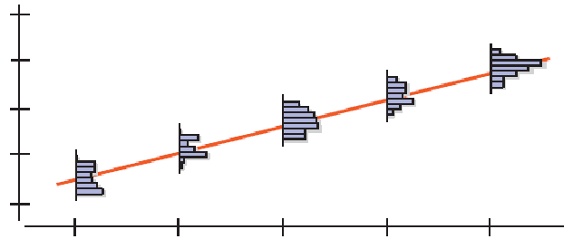
We can account for the difference between $\hat{y}$ and $\mu_y$ by adding the error residual, or $\varepsilon$:
Degrees of Freedom
Let us compute degrees of freedom for all three $SS$ in the regression ANOVA.
The total sum of squares $SS_{TOT}$ has $df_{TOT} = n-1$ degrees of freedom because it comesdirectly from the sample variance $s^2_y$.
The regression sum of squares $SS_{REG}$ has $df_{REG} = 1$.
For $df_{ERR} = n-2$ degrees of freedom for the error sum of squares, so that
Variance Estimation
The standard deviation of the residuals, $s_e$, gives us a measure of how much the points spread around the regression line.
The spread of the residuals is about the same everywhere, and standard deviation around the line should be the same.
|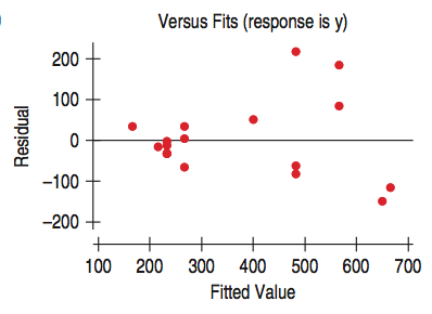 |It appears that the spread in the residuals is increasing.| |-|-|
ANOVA Table
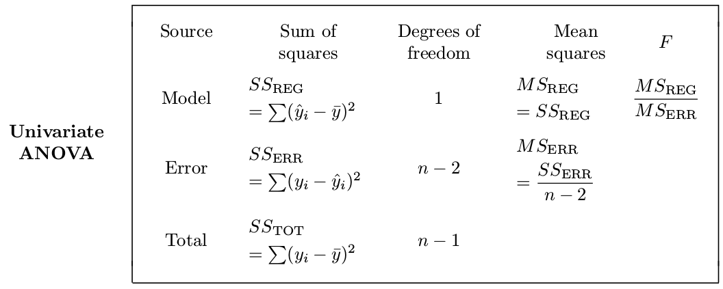
Regression Variance
Mean squares $MS_{REG}$ and $MS_{ERR}$ are obtained from the corresponding sums of squares dividing them by their degrees of freedom.
The estimated standard deviation $s$ is usually called root mean squared error or RMSE.
The F-ratio
is used to test significance of the entire regression model.
Assumptions and Conditions for ANOVA
Independence Assumption
The groups must be independent of each other.
No test can verify this assumption. You have to think about how the data were collected and check that the Randomization Condition is satisfied.
Equal Variance Assumption
ANOVA assumes that the true variances of the treatment groups are equal. We can check the corresponding Similar Variance Condition in various ways:
Look at side-by-side boxplots of the groups. Look for differences in spreads.
Examine the boxplots for a relationship between the mean values and the spreads. A common pattern is increasing spread with increasing mean.
Look at the group residuals plotted against the predicted values (group means). See if larger predicted values lead to larger-magnitude residuals.
Normal Population Assumption
Like Student's t-tests, the F-test requires that the underlying errors follow a Normal model. As before when we faced this assumption, we'll check a corresponding Nearly Normal Condition.
Examine the boxplots for skewness patterns.
Examine a histogram of all the residuals.
Example a Normal probability plot.
Regression Inference
Collect a sample and estimate the population $\beta$'s by finding a regression line:
where $b_0$ estimates $\beta_0$, $b_1$ estimates $\beta_1$.
The residuals $e = y - \hat{y}$ are the sample based versions of $\varepsilon$.
Account for the uncertainties in $\beta_0$ and $\beta_1$ by making confidence intervals, as we've done for means and proportions.
Assumptions and Conditions
The inference methods are based on these assumptions:
Linearity Assumption: This condition is satisfied if the scatterplot of $x$ and $y$ looks straight.
Independence Assumption: Look for randomization in the sample or the experiment. Also check the residual plot for lack of patterns.
Equal Variance Assumption: Check the Equal Spread Condition, which means the variability of $y$ should be about the same for all values of $x$.
Normal Population Assumption: Assume the errors around the idealized regression line at each value of $x$ follow a Normal model. Check if the residuals satisfy the Nearly Normal Condition.
Assumptions and Conditions (cont.)
Summary of Assumptions and Conditions:
Make a scatterplot of the data to check for linearity. (Linearity Assumption)
Fit a regression, find the residuals, $e$, and predicted values $\hat{y}$.
Plot the residuals against time (if appropriate) and check for evidence of patterns (Independence Assumption).
Make a scatterplot of the residuals against x or the predicted values. This plot should not exhibit a "fan" or "cone" shape. (Equal Variance Assumption)
Make a histogram and Normal probability plot of the residuals (Normal Population Assumption)
The Standard Error of the Slope
For a sample, we expect $b_1$ to be close, but not equal to the model slope $\beta_1$.
For similar samples, the standard error of the slope is a measure of the variability of $b_1$ about the true slope $\beta_1$.
where $s_e$ is spread around the line, $s_x$ is spread of $x$ values, $n$ is a sample size.
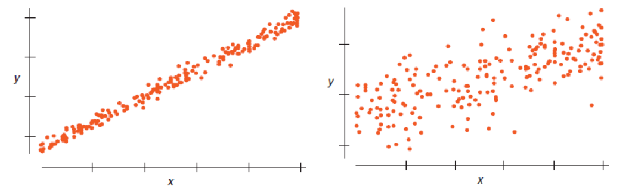
Example 5
Which of these scatterplots would give the more consistent regression slope estimate if we were to sample repeatedly from the underlying population?
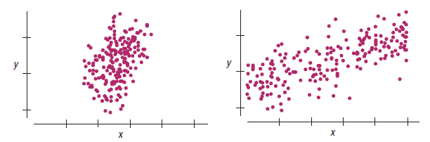
Example 6
Which of these scatterplots would give the more consistent regression slope estimate if we were to sample repeatedly from the underlying population?
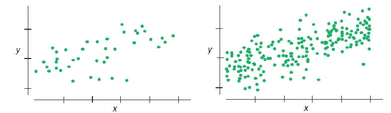
Example 7
Which of these scatterplots would give the more consistent regression slope estimate if we were to sample repeatedly from the underlying population?
A Test for the Regression Slope
When the conditions are met, the standardized estimated regression slope,
follows a Student's t-model with $n - 2$ degrees of freedom. We calculate the standard error as SE (see above), where $s_e = \sqrt{\frac{\sum(y-\hat{y})^2}{n-2}}$ and $s_x$ is the standard deviation of the $x$-values.
A Test for the Regression Slope (cont.)
When the assumptions and conditions are met, we can test the hypothesis $H_0: \beta_1 = B_1$ vs. $H_A: \beta_1 \ne B_1$ using the standardized estimated regression slope,
follows a Student's $t$-model with $n - 2$ degrees of freedom.
We can use the $t$-model to find the P-value of the test.
CI for the Regression Slope
When the assumptions and conditions are met, we can find a confidence interval for $\beta_1$ from
where the critical value $t^*$ depends on the confidence level and has $n - 2$ degrees of freedom.
ANOVA F-test
It compares the portion of variation explained by regression with the portion that remains unexplained.
F-statistic is a ratio of two quantities that are that are expected to be roughly equal under the null hypothesis, which is approximately 1.
Each portion of the total variation is measured by the corresponding sum of squares. Dividing each $SS$ by the number of degrees of freedom, we obtain mean squares,
Under null hypothesis $H_0: \beta_1 = 0$, both means are independent, and their ratio
has F-distribution with $df_{REG} = 1$ and $df_{ERR} = n - 2$.
A Hypothesis Test for Correlation
What if we want to test whether the correlation between $x$ and $y$ is 0?
When the conditions are met, we can test the hypothesis $H_0 : r = 0$ vs. $H_A : r \ne 0$ using the test statistic:
which follows a Student's $t$-model with $n - 2$ degrees of freedom.
We can use the $t$-model to find the P-value of the test.
F-test and T-test
The T-test for the regression slope and the ANOVA F-test for the univariate regression, they are absolutely equivalent.
Prediction
Let $x_*$ be the value of the predictor $X$. The corresponding value of the response $Y$ is
How reliable are regression predictions, and how close are they to the real true values? We can construct
a $(1-\alpha)100\%$ confidence interval for the expectation $\mu_* = E(Y | X=x_*)$
a $(1-\alpha)100\%$ prediction interval for the expectation for $Y = y_*$ when $X=x_*$
The Confidence Interval for the Mean Response
When the conditions are met, we find the confidence interval for the mean response value $\mu_*$ at a value $x_*$ as
where the standard error is
The Prediction Interval for an Individual Response
When the conditions are met, we can find the prediction interval for all values of $y_*$ at a value $x_*$ as
where the standard error is