Bayesian Inference

Bayesian approach

There is a difference in our treatment of uncertainty.

Frequentist approach: all probabilities refer to random samples of data and possible long-run frequencies, and so do such concepts as unbiasedness, consistency, confidence level, and significance level.

Bayesian approach: Uncertainty is also attributed to the unknown parameter $\theta$, but some values of $\theta$ are more likely than others. It reflects our ideas, beliefs, and past experiences about the parameter before we collect and use the data.

Prior distribution is whole distribution of values of $\theta$.

Example 1

What do you think is the average starting annual salary of a Computer Science graduate? We can certainly collect data and compute an estimate of average salary.

Before that, we already have our beliefs on what the mean salary may be. We can express it as some distribution with the most likely range between 40,000 and 70,000.

Collected data may force us to change our initial idea about the unknown parameter.

Probabilities of different values of of $\theta$ may change. Then we'll have a posterior distribution of of $\theta$.

Prior and Posterior

There are two sources of information to use in Bayesian inference:

collected and observed data;
prior distribution of the parameter.

Prior to the experiment, our knowledge about the parameter $\theta$ is expressed in terms of the prior distribution, $\pi(\theta)$.

The observed sample of data $X = (X_1, \ldots, X_n)$ has distribution

\[f(x|\theta) = f(x_1, \ldots, x_n|\theta)\]

Observed data add information about the parameter, so the updated knowledge about $\theta$ can be expressed as the posterior distribution.

\[\pi(\theta|x) = \pi(\theta| X = x) = \frac{f(x|\theta)\pi(\theta)}{m(x)}\]

Marginal Distribution

The denominator, $m(x)$, represents the unconditional distribution of data $X$. This is the marginal distribution of the sample $X$.

Being unconditional means that it is constant for different values of the parameter $\theta$. It can be computed by the Law of Total Probability or its continuous-case version.

\[m(x) = \sum_{\theta} f(x|\theta)\pi(\theta)\]

\[m(x) = \int_{\theta} f(x|\theta)\pi(\theta) d\theta\]

Example 2

A manufacturer claims that the shipment contains only 5% of defective items, but the inspector feels that in fact it is 10%. We have to decide whether to accept or to reject the shipment based on $\theta$, the proportion of defective parts.

Before we see the real data, let's assign a 50-50 chance to both suggested values of $\theta$, i.e., $\pi(0.05) = \pi(0.10) = 0.5$.

A random sample of 20 parts has 3 defective ones. Calculate the posterior distribution of $\theta$.

Conjugate Distribution Families

A family of prior distributions $\pi$ is conjugate to the model $f(x|\theta)$ if the posterior distribution belongs to the same family.

A suitably chosen prior distribution of $\theta$ may lead to a very tractable form of the posterior.

Gamma Conjugate Prior

Gamma family is conjugate to the Poisson model.

Let $(X_1, \ldots, X_n)$ be a sample from $Poisson(\theta)$ distribution with a $Gamma(\alpha, \lambda)$ prior distribution of $\theta$.

\[f(x|\theta) = \prod^n_{i=1} f(x_i|\theta) = \prod^n_{i=1} \frac{e^{-\theta}\theta^{x_i}}{x_i!} \sim e^{-n\theta}\theta^{\sum x_i}\]

The Gamma prior distribution of $\theta$ has density

\[\pi(\theta) \sim \theta^{\alpha-1} e^{-\lambda \theta}\]

Then, the posterior distribution of $\theta$ given

\[\pi(\theta|x) \sim f(x|\theta)\pi(\theta) \sim \left( e^{-n\theta}\theta^{\sum x_i} \right) \left(\theta^{\alpha-1} e^{-\lambda \theta} \right)\]

\[\sim \theta^{\alpha+\sum x_i-1} e^{-(\lambda+n)\theta}\]

Gamma Conjugate Prior (cont.)

Comparing with the general form of a $Gamma$ density, we see that $\pi(\theta|x)$ is the $Gamma$ distribution with new parameters,

\[\alpha_x = \alpha +\sum^n_{i=1} x_i\]

and

\[\lambda_x = \lambda + n\]

Example 3

The number of network blackouts each week has $Poisson(\theta)$ distribution. The weekly rate of blackouts $\theta$ is not known exactly, but according to the past experience with similar networks, it averages 4 blackouts with a standard deviation of 2.

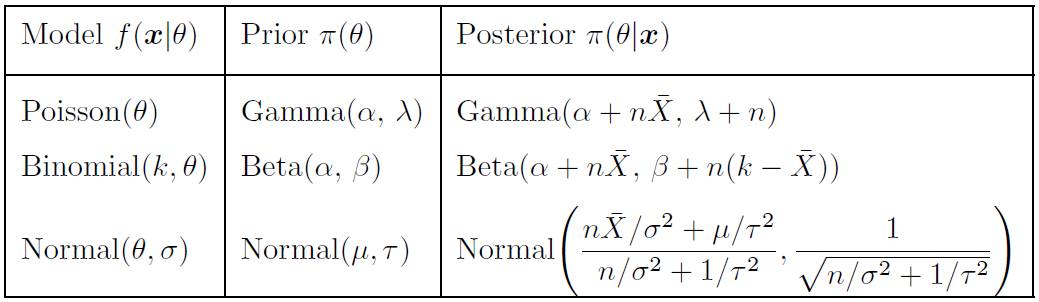
Classical Conjugate Families

conjugate

Bayesian Estimation

To estimate $\theta$, we simply compute the posterior mean,

\[\hat{\theta}_B = E\{\theta|X=x\} = \begin{cases} \sum_\theta \theta \pi(\theta|x) = \frac{\sum \theta f(x|\theta) \pi(\theta)}{\sum f(x|\theta) \pi(\theta)}\\ \int_\theta \theta \pi(\theta|x) = \frac{\int \theta f(x|\theta) \pi(\theta)}{\int f(x|\theta) \pi(\theta)} \end{cases}\]

The result is a conditional expectation of $\theta$ given data $X$. In abstract terms, the Bayes estimator $\hat{\theta}_B$ is what we "expect" $\theta$ to be, after we observed a sample.

Accuracy

Estimator $\hat{\theta}_B = E\{\theta|x\}$ has the lowest squared-error posterior risk

\[\rho(\hat{\theta}_B) = E \{(\hat{\theta} - \theta)^2 | X=x\}\]

For the Bayes estimator $\hat{\theta}_B$, posterior risk equals posterior variance.

\[\rho(\hat{\theta}_B) = E \{(E\{\theta|x\} - \theta)^2 | x\} = Var\{\theta|x\}\]

which measures variability of $\theta$ around $\hat{\theta}_B$, according to the posterior distribution of $\theta$.

\[P\{\theta \in C| X=x \} = \int_C \pi(\theta|x) d\theta = 1 - \alpha\]

By minimizing the length of set $C$ we get highest posterior density credible set.

\[C = \{\theta | \pi(\theta|x) \geq c \}\]

For the $Normal(\mu_x, \tau_x)$ posterior distribution of $\theta$, the $(1-\alpha)100\%$ HPD set is

\[\mu_x \pm z_{\alpha/2} \tau_x\]

Example 6

Find the HPD set for Example 1.