Continuous Distributions
Probability Density
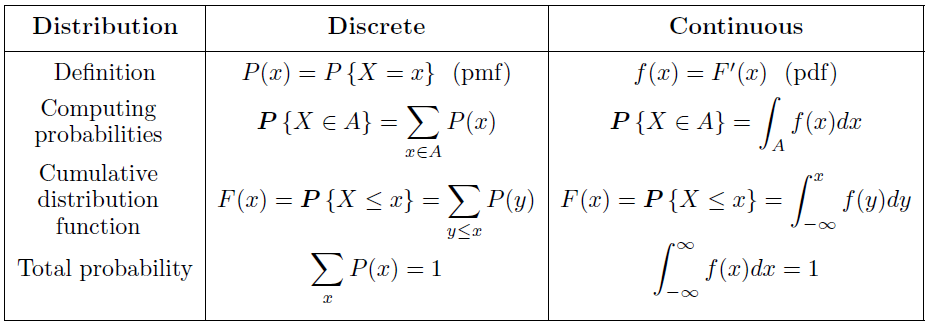
For all continuous variables, the probability mass function (pmf) is always equal to zero, $\forall x \; P(x)=0$
We can use the cumulative distribution function (cdf) $F(x)$. In the continuous case, it equals $F(x) = P \{X \leq x\} = P \{X < x\}$
Assume, additionally, that $F(x)$ has a derivative.
Probability Density Function
Probability density function (pdf, density) is the derivative of the cdf, $f(x) = F'(x)$. The distribution is called continuous if it has a density.
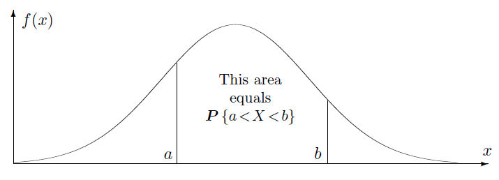
Then, $F(x)$ is an antiderivative of a density, so the integral of a density from $a$ to $b$ equals to the difference of antiderivatives, i.e.,
Example 1
The lifetime, in years, of some electronic component is a continuous random variable with the density
Find $k$, and compute the probability for the lifetime to exceed 5 years.
PMF vs PDF
Joint and Marginal Densities
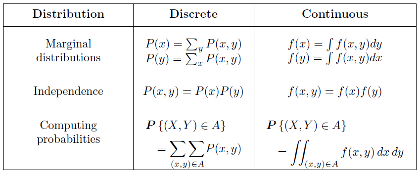
For a vector of random variables, the joint cumulative distribution function is defined as
The joint density is the mixed derivative of the joint cdf,
Marginal density of $X$ or $Y$ can be obtained by integrating out the other variable.
Variables $X$ and $Y$ are independent if their joint density factors into the product of marginal densities.
Joint and Marginal Densities (cont.)
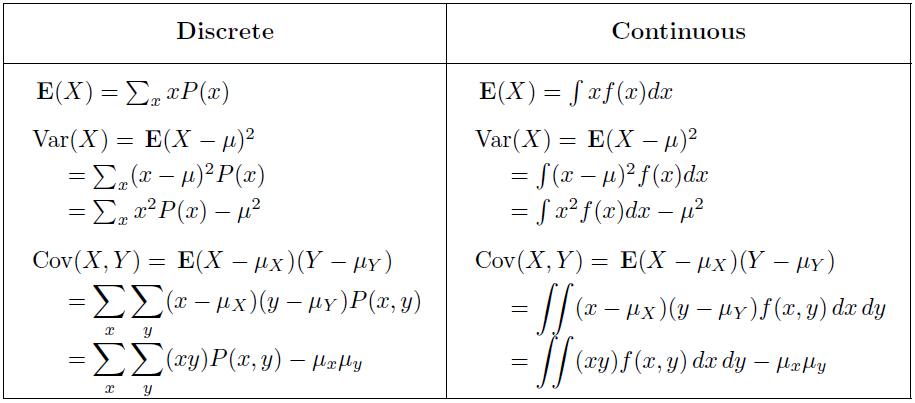
Expectation and Variance
Example 2
A random variable $X$ in Example 1 has density $f(x) = 2x^{-3} \text{ for } x \geq 1$
What is its expectation?
Uniform Distribution
The Uniform distribution has a constant density, $f(x) = \frac{1}{b-a}, a < x < b$
For any $h>0$ and $t \in [a, b-h]$, the probability is independent of $t$. $P\{ t < X < t+h \} = \int_t^{t+h} \frac{1}{b-a}dx = \frac{h}{b-a}$
Uniform property: the probability is only determined by the length of the interval, but not by its location.
Standard Uniform Distribution
The Uniform distribution with $a = 0$ and $b = 1$ is called Standard Uniform distribution.
Its density is $f(x) = 1$ for $0 < x < 1$
If $X$ is a Uniform(a, b) random variable, then
is Standard Uniform. Likewise, if $Y$ is Standard Uniform, then
is Uniform(a, b).
Expectation and Variance
For a Standard Uniform variable $Y$,
Expectation and Variance (cont.)
Let $X = a+(b-a)Y$ which has a Uniform(a, b) distribution, so
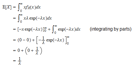
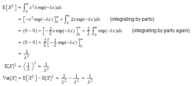
Exponential Distribution
Exponential distribution is often used to model time.
The quantity $\lambda$ is a parameter of Exponential distribution, and its meaning is clear from $E(X)$.
Example 3
Jobs are sent to a printer at an average rate of 3 jobs per hour.
What is the expected time between jobs?
What is the probability that the next job is sent within 5 minutes?
Memoryless Property
Memoryless property: Exponential variables lose memory
It means that the fact of having waited for $t$ minutes gets "forgotten", and it does not affect the future waiting time.
Regardless of the event $T > t$, when the total waiting time exceeds $t$, the remaining waiting time still has Exponential distribution with the same parameter. $P\{T > t+x | T>t\} = P\{T>x\} \text{ for } t,x >0$
Gamma Distribution
When a certain procedure consists of $\alpha$ independent steps, and each step takes Exponential($\lambda$) amount of time, then the total time has Gamma distribution with parameters $\alpha$ and $\lambda$.
where
When $\alpha = 1$, the Gamma distribution becomes Exponential.
When $\lambda = 1/2$ and $\alpha > 0$, the Gamma distribution becomes Chi-square with $2\alpha$ degrees of freedom.
Expectation and Variance
Gamma-Poisson Formula
Let $T$ be a Gamma variable with an integer parameter $\alpha$ and some positive $\lambda$.
This is a distribution of the time of the $\alpha$-th rare event.
Then, the event $\{T > t\}$ means that the $\alpha$-th rare event occurs after the moment $t$.
fewer than $\alpha$ rare events occur before the time $t$.
where $X$ has Poisson distribution with parameter $\lambda t$.
Example 4
Lifetimes of computer memory chips have Gamma distribution with expectation $\mu = 12$ years and standard deviation $\sigma = 4$ years.
What is the probability that such a chip has a lifetime between 8 and 10 years?
Normal Distribution
Normal distribution is often found to be a good model for physical variables. It has density
Standard Normal Distribution
Normal distribution with "standard parameters" $\mu = 0$ and $\sigma = 1$ is called Standard Normal distribution.
Example 5
For a Standard Normal random variable $Z$, find
P{Z < 1.35}
P{Z > 1.35}
P{-0.77 < Z < 1.35}
Central Limit Theorem
Let $X_1, X_2, \ldots$ be independent random variables with the same expectation $\mu = E(X_i)$ and standard deviation $\sigma = Std(X_i)$, and let
As $n \rightarrow \infty$, the standardized sum
converges in distribution to a SN random variable for all $z$, s.t. $F_{Z_n}(z) = P \left \{ \frac{S_n - n\mu}{\sigma \sqrt n} \leq z \right \} \rightarrow \Phi(z)$
Example 6
A disk has free space of 330 megabytes. Is it likely to be sufficient for 300 independent images, if each image has expected size of 1 megabyte with a standard deviation of 0.5 megabytes?
The Normal Approximation for the Binomial
Sum of many independent 0/1 components with probabilities equal $p$ (discrete Binomial model) is approximately Normal with
if we expect at least 10 successes and 10 failures:
Example 6
Suppose the probability of finding a prize in a cereal box is 20%. If we open 50 boxes, then the number of prizes found is a Binomial distribution with mean of 10:
For Binomial(50, 0.2), $\mu = 10$ and $\sigma = 2.83$
To estimate P(10):