Lecture 10
Outline
Inference for Regression
Inference for Regression
The Population and the Sample
But we know observations vary from sample to sample. So we imagine a true line that summarizes the relationship between x and y for the entire population,
Where $\mu_y$ is the population mean of $y$ at a given value of $x$.
We write $\mu_y$ instead of $y$ because the regression line assumes that the means of the $y$ values for each value of $x$ fall exactly on the line.
The Population and the Sample (cont.)
For a given value x:
Most, if not all, of the y values obtained from a particular sample will not lie on the line.
The sampled y values will be distributed about $\mu_y$.
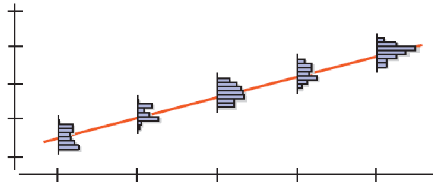
We can account for the difference between $\hat{y}$ and $\mu_y$ by adding the error residual, or $\varepsilon$:
Regression Inference
Collect a sample and estimate the population $\beta$'s by finding a regression line:
where $b_0$ estimates $\beta_0$, $b_1$ estimates $\beta_1$.
The residuals $e = y - \hat{y}$ are the sample based versions of $\varepsilon$.
Account for the uncertainties in $\beta_0$ and $\beta_1$ by making confidence intervals, as we've done for means and proportions.
Assumptions and Conditions
The inference methods are based on these assumptions:
Linearity Assumption: This condition is satisfied if the scatterplot of $x$ and $y$ looks straight.
Independence Assumption: Look for randomization in the sample or the experiment. Also check the residual plot for lack of patterns.
Equal Variance Assumption: Check the Equal Spread Condition, which means the variability of $y$ should be about the same for all values of $x$.
Normal Population Assumption: Assume the errors around the idealized regression line at each value of $x$ follow a Normal model. Check if the residuals satisfy the Nearly Normal Condition.
Assumptions and Conditions (cont.)
Summary of Assumptions and Conditions:
Make a scatterplot of the data to check for linearity. (Linearity Assumption)
Fit a regression, find the residuals, $e$, and predicted values $\hat{y}$.
Plot the residuals against time (if appropriate) and check for evidence of patterns (Independence Assumption).
Make a scatterplot of the residuals against x or the predicted values. This plot should not exhibit a "fan" or "cone" shape. (Equal Variance Assumption)
Make a histogram and Normal probability plot of the residuals (Normal Population Assumption)
The Standard Error of the Slope
For a sample, we expect $b_1$ to be close, but not equal to the model slope $\beta_1$.
For similar samples, the standard error of the slope is a measure of the variability of $b_1$ about the true slope $\beta_1$.
where $s_e$ is spread around the line, $s_x$ is spread of $x$ values, $n$ is a sample size.
Example 1
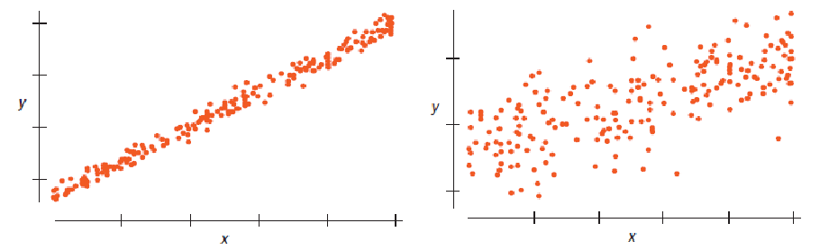
Which of these scatterplots would give the more consistent regression slope estimate if we were to sample repeatedly from the underlying population?
Example 2
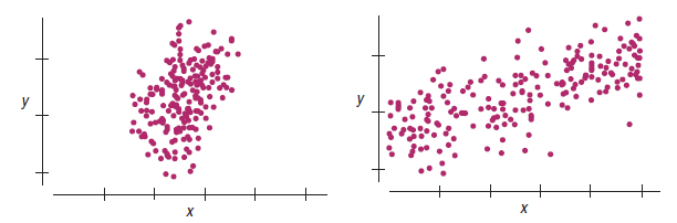
Which of these scatterplots would give the more consistent regression slope estimate if we were to sample repeatedly from the underlying population?
Example 3
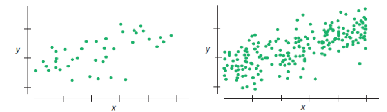
Which of these scatterplots would give the more consistent regression slope estimate if we were to sample repeatedly from the underlying population?
A Test for the Regression Slope
When the conditions are met, the standardized estimated regression slope,
follows a Student's t-model with $n - 2$ degrees of freedom. We calculate the standard error as SE (see above), where $s_e = \sqrt{\frac{\sum(y-\hat{y})^2}{n-2}}$ and $s_x$ is the standard deviation of the $x$-values.
A Test for the Regression Slope
When the assumptions and conditions are met, we can test the hypothesis $H_0: \beta_1 = 0$ vs. $H_A: \beta_1 \ne 0$ using the standardized estimated regression slope,
follows a Student's $t$-model with $n - 2$ degrees of freedom.
We can use the $t$-model to find the P-value of the test.
A Test for the Regression Slope
When the assumptions and conditions are met, we can find a confidence interval for $\beta_1$ from $b_1 \pm t^*_{n-2} * SE(b_1)$
where the critical value $t^*$ depends on the confidence level and has $n - 2$ degrees of freedom.
A Hypothesis Test for Correlation
What if we want to test whether the correlation between $x$ and $y$ is 0?
When the conditions are met, we can test the hypothesis $H_0 : r = 0$ vs. $H_A : r \ne 0$ using the test statistic:
which follows a Student's $t$-model with $n - 2$ degrees of freedom.
We can use the $t$-model to find the P-value of the test.
The Confidence Interval for the Mean Response
When the conditions are met, we find the confidence interval for the mean response value $\mu_v$ at a value $x_v$ as
where the standard error is
The Prediction Interval for an Individual Response
When the conditions are met, we can find the prediction interval for all values of $y$ at a value $x_v$ as
where the standard error is