Lecture 3
Outline
Linear Regression
Randomness and Probability Models
The Linear Model
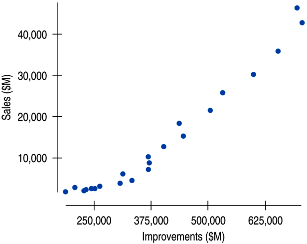
The scatterplot below shows Lowe's sales and home improvement expenditures between 1985 and 2007.
The relationship is strong, positive, and linear (r = 0.976).
The Linear Model (cont.)
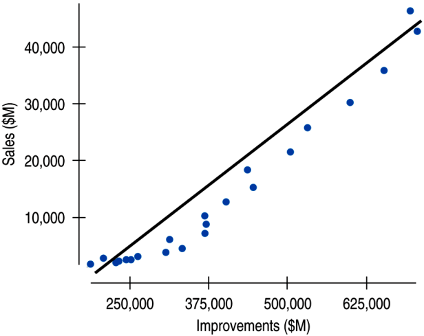
We see that the points don't all line up, but that a straight line can summarize the general pattern. We call this line a linear model.
A linear model describes the relationship between x and y.
Residuals
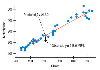
A linear model can be written in the form $\hat{y} = b_0 + b_1x$ where $b_0$ and $b_1$ are numbers estimated from the data and $\hat{y}$ is the predicted value.
The difference between the predicted value and the observed value, $y$, is called the residual and is denoted $e$.
Example
In the computer usage model for 301 stores, the model predicts 262.2 MIPS (Millions of Instructions Per Second) and the actual value is 218.9 MIPS. We may compute the residual for 301 stores.
Best Fit
The line of best fit is the line for which the sum of the squared residuals is smallest - often called the least squares line.
Example: Pizza Sales and Price
A linear model to predict weekly Sales of frozen pizza (in pounds) from the average price (dollars/unit) charged by a sample of stores in Dallas in 39 recent weeks is
What is the explanatory variable?
What is the response variable?
What does the slope mean in this context?
Is the y-intercept meaningful in this context?
What is the predicted Sales if the average price charged was $3.50 for a pizza?
If the sales for a price of $3.50 turned out to be 60,000 pounds, what would the residual be?
Correlation and the Line
We can find the slope of the least squares line using the correlation and the standard deviations.
The slope gets its sign from the correlation.
The slope gets its units from the ratio of the two standard deviations.
Correlation and the Line (cont.)
To find the intercept of our line, we use the means. If our line estimates the data, then it should predict $\bar{y}$ for the x-value.
Example: Carbon Footprint
Understanding Regression from Correlation
If we consider finding the least squares line for standardized variables $z_x$ and $z_y$, the formula for slope can be simplified.
From above we see that for an observation 1 SD above the mean in $x$, you'd expect $y$ to have a z-score of $r$.
Regression to the Mean
The previous equation shows that if $x$ is 2 SDs above its mean, we won't ever move more than 2 SDs away for $y$, since $r$ can't be bigger than 1.
So, each predicted $y$ tends to be closer to its mean than its corresponding $x$ was.
This property of the linear model is called regression to the mean.
Checking the Model
Models are useful only when specific assumptions are resonable:
Quantitative Data Condition – linear models only make sense for quantitative data, so don't be fooled by categorical data recorded as numbers.
Linearity Assumption check Linearity Condition – two variables must have a linear association, or a linear model won't mean a thing.
Outlier Condition – outliers can dramatically change a regression model.
Equal Spread Condition – check a residual plot for equal scatter for all x-values.
Checking the Model (cont.)
The standard deviation of the residuals, $s_e$, gives us a measure of how much the points spread around the regression line.
The spread of the residuals is about the same everywhere, and standard deviation around the line should be the same.
|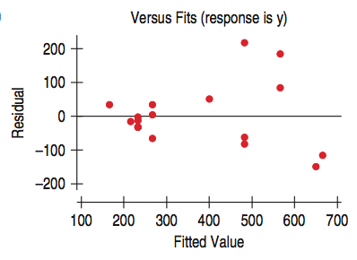 |It appears that the spread in the residuals is increasing.| |-|-|
Variation in the Model
The variation in the residuals shows how well a model fits
If the correlation were 1, then the model predicts $y$ perfectly, the residuals would all be zero and have no variation.
If the correlation were 0, the model would predict the mean for all x-values. The residuals would have the same variability as the original data.
Consider the square of the correlation coefficient $r$ to get $r^2$ which is a value between 0 and 1.
- \[r^2\]
gives the fraction of the data's variation accounted for by the model
- \[1-r^2\]
is the fraction of the original variation left in the residuals.
Nonlinear Relationships
| Plot | Description |
|---|---|
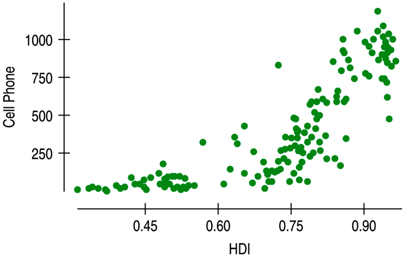 | A nonlinear relationship that is not appropriate for linear regression. |
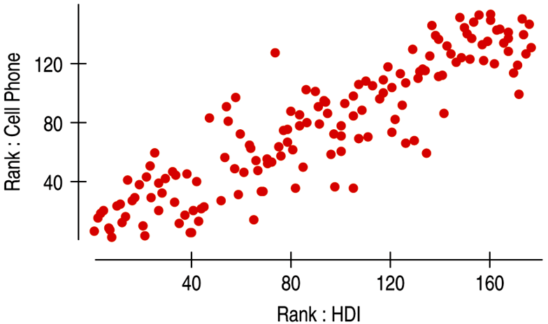 | The Spearman rank correlation works with the ranks of data, but a linear model is difficult to interpret so it’s not appropriate. |
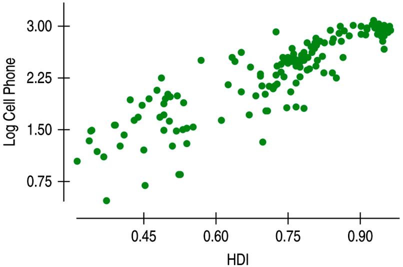 | Transforming or re-expresing one or both variables by a function such as square root, logarithm, etc. Though some times difficult to interpret, regression models and supporting statistics are useful. |
Randomness and Probability Models
Random phenomena
Sample space is a special event that is the collection of all possible outcomes.
Denoted as $S$ or sometimes $\Omega$.
The probability of an event is its long-run relative frequency.
Independence means that the outcome of one trial doesn't influence or change the outcome of another.
Law of Large Numbers
The Law of Large Numbers (LLN) states that if the events are independent, then as the number of trials increases, the long-run relative frequency of an event gets closer and closer to a single value.
Empirical probability is based on repeatedly observing the event's outcome.
Probability
The (theoretical) probability of event A can be computed as
Probability Rules
If the probability of an event occurring is 0, the event can't occur.
If the probability is 1, the event always occurs.
For any event A, $0 \leq P(A) \leq 1$.
The probability of the set of all possible outcomes must be 1, $P(S)=1$.
The probability of an event occurring is 1 minus the probability that it doesn't occur, $P(A)=1-P(A^c)$.
Example
Lee's Lights sell lighting fixtures. Lee records the behavior of 1000 customers entering the store during one week. Of those, 300 make purchases. What is the probability that a customer doesn't make a purchase?
Probability Rules (cont.)
For two independent events A and B, the probability that both A and B occur is the product of the probabilities of the two events.
where A and B are independent.
Example
Whether or not a caller qualifies for a platinum credit card is a random outcome. Suppose the probability of qualifying is 0.35. What is the chance that the next two callers qualify?
Probability Rules (cont.)
The probability of disjoint events to occur is the sum of the probabilities that such events.
Two events are disjoint (or mutually exclusive) if they have no outcomes in common.
where A and B are disjoint.
Example
Some customers prefer to see the merchandise but then make their purchase online. Lee determines that there's an 8% chance of a customer making a purchase in this way. We know that about 30% of customers make purchases when they enter the store. What is the probability that a customer who enters the store makes no purchase at all?
Probability Rules (cont.)
The General Addition Rule calculates the probability that either of two events occurs. It does not require that the events be disjoint.
Example
Lee notices that when two customers enter the store together, their behavior isn't independent. In fact, there's a 20% they'll both make a purchase. When two customers enter the store together, what is the probability that at least one of them will make a purchase?
Example
You and a friend get your cars inspected. The event of your car's passing inspection is independent of your friend's car. If 75% of cars pass inspection what is the probability that
Your car passes inspection?
Your car doesn't pass inspection?
Both cars pass inspection?
At least one of two cars passes?
Neither car passes inspection?
Contingency Tables
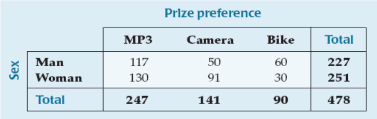
Marginal probability depends only on totals found in the margins of the table.
Joint probabilities give the probability of two events occurring together.
Conditional Probability
A probability that takes into account a given condition is called a conditional probability.
General Multiplication Rule calculates the probability that both of two events occurs. It does not require that the events be independent.
Example
What is the probability that a randomly selected customer wants a bike if the customer selected is a woman?
Are "Prize preference" and "Sex" independent?