Lecture 5
Outline
Normal Distribution
Sampling Distribution
Central Limit Theorem
Normal Distribution
The 68-95-99.7 Rule
A z-score reports the number of standard deviations away from the mean.
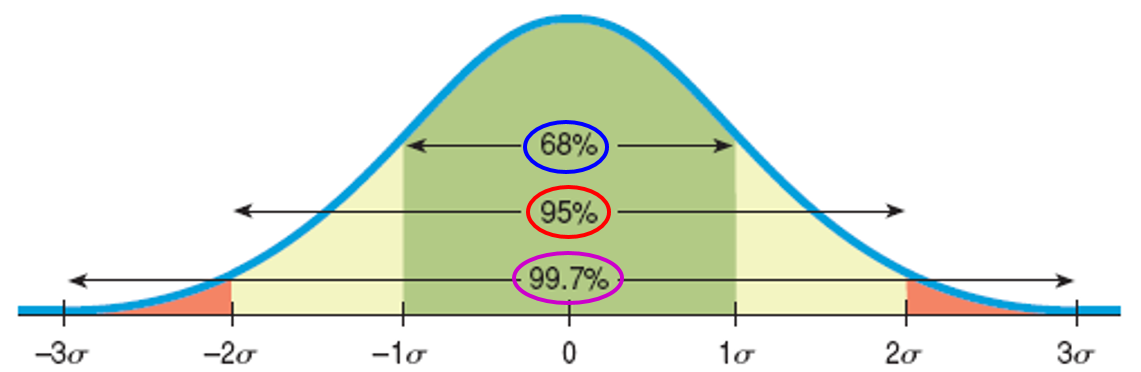
In bell-shaped distributions, about 68% of the values fall within one standard deviation of the mean, about 95% of the values fall within two standard deviations of the mean, and about 99.7% of the values fall within three standard deviations of the mean.
The Normal Distribution
The model for symmetric, bell-shaped, unimodal histograms is called the Normal model.
We write N($\mu$,$\sigma$) to represent a Normal model with mean $\mu$ and standard deviation $\sigma$.
The model with mean 0 and standard deviation 1 is called the standard Normal model (or the standard Normal distribution). This model is used with standardized z-scores.
Example 1
Each Scholastic Aptitude Test (SAT) has a distribution that is roughly unimodal and symmetric and is designed to have an overall mean of 500 and a standard deviation of 100.
Suppose you earned a 600 on an SAT test. From the information above and the 68-95-99.7 Rule, where do you stand among all students who took the SAT?
Example 1 (cont.)
Because we’re told that the distribution is unimodal and symmetric, with a mean of 500 and an SD of 100, we’ll use a N(500,100) model.
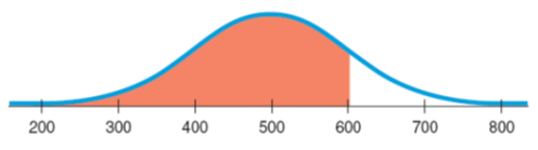
A score of 600 is 1 SD above the mean. That corresponds to one of the points in the 68-95-99.7% Rule.
About 32% (100% – 68%) of those who took the test were more than one SD from the mean, but only half of those were on the high side.
So about 16% (half of 32%) of the test scores were better than 600.
Example 2
Assuming the SAT scores are nearly normal with N(500,100), what proportion of SAT scores falls between 450 and 600?
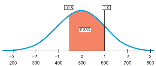
Using a table or calculator, we find the area z ≤ 1.0 = 0.8413, which means that 84.13% of scores fall below 1.0, and the area z ≤ –0.50 = 0.3085, which means that 30.85% of the values fall below –0.5.
The proportion of z-scores between them is 84.13% – 30.85% = 53.28%. So, the Normal model estimates that about 53.3% of SAT scores fall between 450 and 600.
Example 3
A college says it admits only people with SAT scores among the top 10%. How high an SAT score does it take to be eligible?
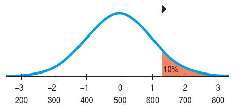
From our picture we can see that the z-value is between 1 and 1.5 (if we’ve judged 10% of the area correctly), and so the cutoff score is between 600 and 650 or so.
Exmple 4
A tire manufacturer believes that the tread life of its snow tires can be described by a Normal model with a mean of 32,000 miles and a standard deviation of 2500 miles.
Approximately what percent of these snow tires will last less than 30,000 miles?
Approximately what percent of these snow tires will last between 30,000 and 35,000 miles?
A dealer wants to offer a refund to customers whose snow tires fail to reach a certain number of miles, but he can only offer this to no more than 1 out of 25 customers. What mileage can he guarantee?
Normal Probability Plots
The Normal probability plot is a specialized graph that can help decide whether the Normal model is appropriate.
If the data are approximately normal, the plot is roughly a diagonal straight line.
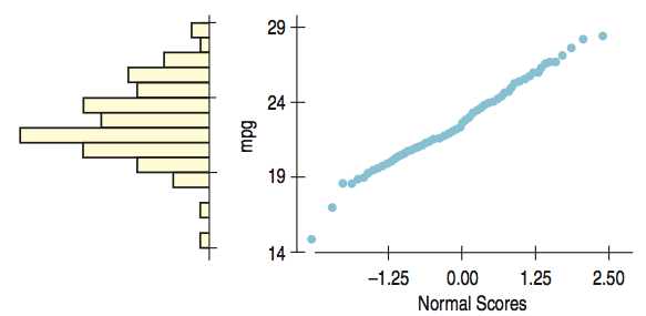
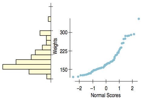
Normal Probability Plots (cont.)
If normal probability plot shows a curve, it reveals skewness (see in the histogram).
Sum of Normal Models
The sum or difference of two independent Normal random variables is also Normal.
Exmple 5
A company that manufactures small stereo systems uses a two-step packaging process.
Stage 1 is combining all small parts into a single packet, $\mu = 9$ and $\sigma = 1.5$ ( in minutes).
Then the packet is sent to Stage 2 where it is boxed, closed, sealed and labeled for shipping, $\mu = 6$ and $\sigma = 1$.
Since both stages are unimodal and symmetric, what is the probability that packing an order of two systems takes more than 20 minutes?
Exmple 5 (cont.)
Normal Model Assumption: We are told both stages are unimodal and symmetric. And we know that the sum of two Normal random variables is also Normal.
Independence Assumption: It is reasonable to think the packing time for one system would not affect the packing time for the next system.
Given:
P1 = time for packing the first system
P2 = time for packing the second system
T = total time to pack two systems, T = P1 + P2
Thus:
E(T) = E(P1 + P2) = E(P1) + E(P2) = 9 + 6 = 15 minutes
- \[Var(P1 + P2) = Var(P1) + Var(P2) = 1.5^2 + 1^2 = 3.25\]
- \[\sigma_T = \sqrt{3.25} = 1.8\]
minutes
Exmple 5 (cont.)
What is the probability that packing an order of two systems takes more than 20 minutes?
We can model the time, T, with a N(15, 3.25) model.
Using past history to build a model, we find slightly more than a 0.3% chance that it will take more than 20 minutes to pack an order of two stereo systems.
The Normal Approximation for the Binomial
A discrete Binomial model is approximately Normal if we expect at least 10 successes and 10 failures:
Example 6
Suppose the probability of finding a prize in a cereal box is 20%. If we open 50 boxes, then the number of prizes found is a Binomial distribution with mean of 10:
For Binomial(50, 0.2), $\mu = 10$ and $\sigma = 2.83$
To estimate P(10):
Sampling Distribution
The Distribution of Sample Proportions
We probably will never know the value of the true proportion, $p$, of an event in the population.
A simulation can help us understand how sample proportions vary due to random sampling.
We set the true proportion of successes to a known value, draw random samples, and then record the sample proportion of successes, which we denote by $\hat{p}$, for each sample.
Even though the $\hat{p}$'s vary from sample to sample, they do so in a way that we can model and understand.
Sampling Distribution for Proportions
The distribution of proportions over many independent samples from the same population is called the sampling distribution of the proportions.
For distributions that are bell-shaped and centered at the true proportion, $p$, we can use the sample size $n$ to find the standard deviation of the sampling distribution:
The difference between sample proportions, referred to as sampling error is just the sampling variability you’d expect to see from one sample to another.
Sampling Distribution Model
The particular Normal model, $N(p, \sqrt \frac{pq}{n})$, is a sampling distribution model for the sample proportion.
We don't need to actually draw many samples and accumulate all those sample proportions.
We can calculate what fraction of the distribution will be found in any region.
It won't work for all situations.
Sampling Distribution Model (cont.)
Assumptions
Independence Assumption: The sampled values must be independent of each other.
Sample Size Assumption: The sample size, n, must be large enough.
Conditions
Randomization Condition: If your data come from an experiment, subjects should have been randomly assigned to treatments.
10% Condition: If sampling has not been made with replacement, then the sample size, $n$, must be no larger than 10% of the population.
Success/Failure Condition: The sample size must be big enough so that both the number of "successes", $np$, and the number of "failures", $nq$, are expected to be at least 10.
Example 7
Information on a packet of seeds claims that the germination rate is 92%. Are conditions met to answer the question,
What is the probability that more than 95% of the 160 seeds in the packet will germinate?
Example 7 (cont.)
Independence: It is reasonable to assume the seeds will germinate independently from each other.
Randomization: The sample of seeds can be considered a random sample from all seeds from this producer.
10% Condition : The packet is less than 10% of all seeds manufactured.
Success/Failure Condition: $np = (0.92*160) = 147.2 > 10$ $nq = (0.05*160) = 12.8 > 10$
Example 7 (cont.)
Information on a packet of seeds claims that the germination rate is 92%. What is the probability that more than 95% of the 160 seeds in the packet will germinate?
Central Limit Theorem
Simulating the Sampling Distribution of a Mean
The results of a simulated 10,000 tosses of fair dice 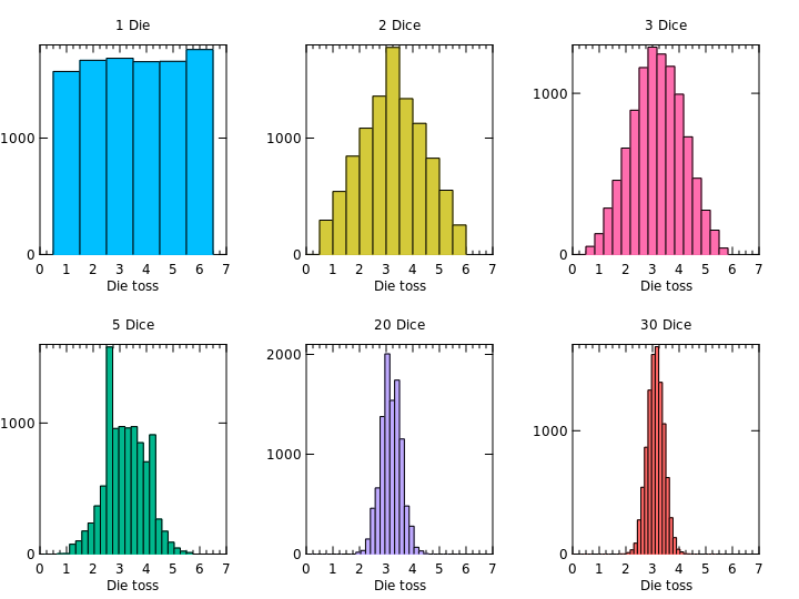
The Central Limit Theorem
Central Limit Theorem (CLT): The mean of a random sample has a sampling distribution whose shape can be approximated by a Normal model. The larger the sample, the better the approxima- tion will be.
The sampling distribution of any mean becomes Normal as the sample size grows.
This is true regardless of the shape of the population distribution!
However, if the population distribution is very skewed, it may take a sample size of dozens or even hundreds of observations for the Normal model to work well.
The Central Limit Theorem (cont.)
The Central Limit Theorem doesn't talk about the distribution of the data from the sample.
It talks about the sample means and sample proportions of many different random samples drawn from the same population.
The Normal model for the sampling distribution of the mean has a standard deviation
where $\sigma$ is the standard deviation of the population.
Assumptions and Conditions for the Sampling Distribution of the Mean
Independence Assumption: The sampled values must be independent of each other.
Sample Size Assumption: The sample size must be sufficiently large.
Randomization Condition: The data values must be sampled randomly, or the concept of a sampling distribution makes no sense.
10% Condition: When the sample is drawn without replacement, the sample size, $n$, should be no more than 10% of the population.
Large Enough Sample Condition: If the population is unimodal and symmetric, even a fairly small sample is okay.
Example 8
According to recent studies, cholesterol levels in healthy U.S. adults average about 215 mg/dL with a standard deviation of about 30 mg/dL and are roughly symmetric and unimodal. If the cholesterol levels of a random sample of 42 healthy U.S. adults is taken, are conditions met to use the normal model?
Randomization
10% Condition
Large Enough Sample Condition
Example 8 (cont.)
Randomization: The sample is random
10% Condition: These 42 healthy U.S. adults are less than 10% of the population of healthy U.S. adults.
Large Enough Sample Condition: Cholesterol levels are roughly symmetric and unimodal so a sample size of 42 is sufficient.
Example 8 (cont.)
What would the mean of the sampling distribution be?
What would the standard deviation of the sampling distribution be?
Example 8 (cont.)
What would the mean of the sampling distribution be?
What would the standard deviation of the sampling distribution be?
What is the probability that the average cholesterol level will be greater than 220?
Law of Diminishing Returns
The standard deviation of the sampling distribution declines only with the square root of the sample size. The square root limits how much we can make a sample tell about the population.