Lecture 11

The Multiple Regression Model

For simple regression, the predicted value depends on only one predictor variable:

\[\hat{y} = b_0 + b_1 x\]

For multiple regression, we write the regression model with more predictor variables:

\[\hat{y} = b_0 + b_1 x_1 + \cdots +b_k x_k\]

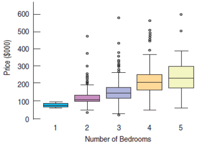
Example 1

Home Price vs. Bedrooms, Saratoga Springs, NY. Random sample of 1057 homes. Can Bedrooms be used to predict Price?

Approximately linear relationship
Equal Spread Condition is violated.
Be cautious about using inferential methods on these data.

mre1

Example 1 (cont.)

mre1

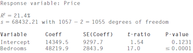
Price = 14,349.5.10 + 48,219.9 Bedrooms
The variation in Bedrooms accounts for only 21% of the variation in Price.
Perhaps the inclusion of another factor can account for a portion of the remaining variation.

Example 1 (cont.)

mre1

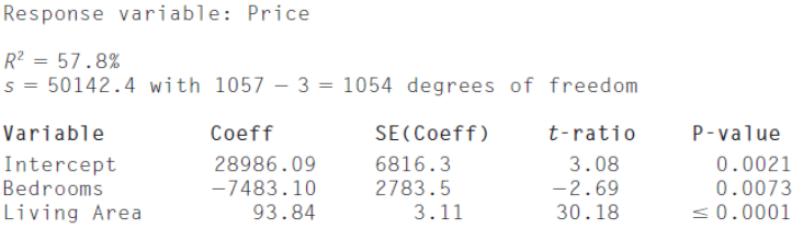
Price = 28,986.10 - 7,483.10 Bedrooms + 93.84 Living Area
Now the model accounts for 58% of the variation in Price.

The Multiple Regression Model (cont.)

Multiple Regression:

Residuals: $e = y - \hat{y}$ (as with simple regression)
Degrees of freedom: $df = n - k -1$
- n = number of observations
- k = number of predictor variables
Standard deviation of residuals:

\[s_e = \sqrt{\frac{\sum(y-\hat{y})^2}{n-k-1}}\]

Interpreting Multiple Regression Coefficients

NOTE: The meaning of the coefficients in multiple regression can be subtly different than in simple regression.

Price = 28,986.10 - 7,483.10 Bedrooms + 93.84 Living Area

Price drops with increasing bedrooms? How can this be correct?

Interpreting Multiple Regression Coefficients (cont.)

In a multiple regression, each coefficient takes into account all the other predictor(s) in the model.

mre1

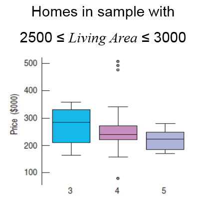
For houses with similar sized Living Areas, more bedrooms means smaller bedrooms and/or smaller common living space. Cramped rooms may decrease the value of a house.

Interpreting Multiple Regression Coefficients (cont.)

So, what's the correct answer to the question:

Do more bedrooms tend to increase or decrease the price of a home?

Correct answer:

"increase" if Bedrooms is the only predictor ("more bedrooms" may mean "bigger house", after all!)
"decrease" if Bedrooms increases for fixed Living Area ("more bedrooms" may mean "smaller, more-cramped rooms")

Summarizing: Multiple regression coefficients must be interpreted in terms of the other predictors in the model.

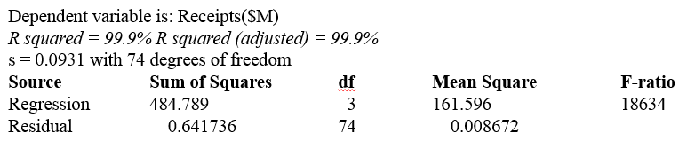
On a typical night in New York City, about 25,000 people attend a Broadway show, paying an average price of more than 75 dollars per ticket. Data for most weeks of 2006-2008 consider the variables Paid Attendance, # Shows, Average Ticket Price(dollars) to predict Receipts. Consider the regression model for these variables.

Interpret the coefficient of Paid Attendance.
Estimate receipts when paid attendance was 200,000 customer attending 30 shows at an average ticket price of 70 dollars.
Is this likely to be a good prediction?
Why or why not?

Example 2 (cont.)

mre5

mre6

Example 2 (cont.)

Write the regression model for these variables.

Receipts = -18.32 + 0.076 Paid Attendance + 0.007 # Shows + 0.24 Average Ticket Price

Interpret the coefficient of Paid Attendance.

If the number of shows and ticket price are fixed, an increase of 1000 customers generates an average increase of $76,000 in receipts.

Estimate receipts when paid attendance was 200,000 customer attending 30 shows at an average ticket price of $70.

$13.89 million

Is this likely to be a good prediction?

Yes, R2 (adjusted) is 99.9% so this model explains most of the variability in Receipts.

Assumptions and Conditions for the Multiple Regression Model

Linearity Assumption

Linearity Condition: Check each of the predictors. Also check the residual plot.

Independence Assumption

Randomization Condition: Does the data collection method introduce any bias?

Equal Variance Assumption

Equal Spread Condition: The variability of the errors should be about the same for each predictor.

Normality Assumption

Nearly Normal Condition: Check to see if the distribution of residuals is unimodal and symmetric.

Assumptions and Conditions

Summary of Multiple Regression Model and Condition Checks:

Check Linearity Condition with a scatterplot for each predictor. If necessary, consider data re-expression.
If the Linearity Condition is satisfied, fit a multiple regression model to the data.
Find the residuals and predicted values.
Inspect a scatterplot of the residuals against the predicted values. Check for nonlinearity and non-uniform variation.
Think about how the data were collected.
- Do you expect the data to be independent?
- Was suitable randomization utilized?
- Are the data representative of a clearly identifiable population?
- Is autocorrelation an issue?

Assumptions and Conditions (cont.)

If the conditions check, feel free to interpret the regression model and use it for prediction.
Check the Nearly Normal Condition by inspecting a residual distribution histogram and a Normal plot. If the sample size is large, the Normality is less important for inference. Watch for skewness and outliers.

Testing the Multiple Regression Model

There are several hypothesis tests in multiple regression
Each is concerned with whether the underlying parameters (slopes and intercept) are actually zero.

The hypothesis for slope coefficients: $H_0: \beta_1 = \beta_2 = \cdots = \beta_k = 0$ $H_A: \text{at least one } \beta \neq 0$

Test the hypothesis with an F-test (a generalization of the t-test to more than one predictor).

Testing the Multiple Regression Model (cont.)

The F-distribution has two degrees of freedom:

\[k\]
, where $k$ is the number of predictors
\[n-k-1\]
, where $n$ is the number of observations

The F-test is one-sided – bigger F-values mean smaller P-values.

If the null hypothesis is true, then F will be near 1.

Testing the Multiple Regression Model (cont.)

If a multiple regression F-test leads to a rejection of the null hypothesis, then check the t-test statistic for each coefficient:

\[t_{n-k-1} = \frac {b_j - 0}{SE(b_j)}\]

Note that the degrees of freedom for the t-test is $n - k - 1$.

Confidence interval:

\[b_j \pm t_{n-k-1}^* \times SE(b_j)\]

Testing the Multiple Regression Model (cont.)

In Multiple Regression, it looks like each $\beta_j$ tells us the effect of its associated predictor, $x_j$.

BUT

The coefficient $\beta_j$ can be different from zero even when there is no correlation between $y$ and $x_j$.
It is even possible that the multiple regression slope changes sign when a new variable enters the regression.

Example 3

On a typical night in New York City, about 25,000 people attend a Broadway show, paying an average price of more than 75 dollars per ticket. The variables Paid Attendance, # Shows, Average Ticket Price(dollars) to predict Receipts.

State hypothesis, the test statistic and p-value, and draw a conclusion for an F-test for the overall model.

Example 3 (cont.)

State hypothesis for an F-test for the overall model.

\[H_0: \beta_1 = \beta_2 = \beta_3 = 0\]

\[H_A: \beta_1 \neq 0, \beta_2 \neq 0, \text{ or } \beta_3 \neq 0\]

State the test statistic and p-value.

mre7

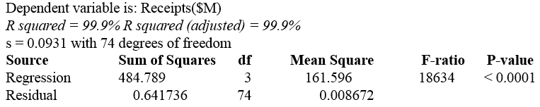
The F-statistic is the F-ratio = 18634. The p-value is < 0.0001.
The p-value is small, so reject the null hypothesis. At least one of the predictors accounts for enough variation in y to be useful.

Example 3 (cont.)

Since the F-ratio suggests that at least one variable is a useful predictor, determine which of the following variables contribute in the presence of the others.

mre8

Paid Attendance (p = 0.0001) and Average Ticket Price (p = 0.0001) both contribute, even when all other variables are in the model.
# Shows however, is not significant (p = 0.116) and should be removed from the model.

Multiple Regression Variation Measures

Summary of Multiple Regression Variation Measures:

Parameters	Significance
$SSE = \sum e^2$	Sum of Squared Residuals: Larger SSE = “noisier” data and less precise prediction
$SSR = \sum (\hat{y} - \bar{y})^2$	Regression Sum of Squares: Larger SSR = stronger model correlation
$SST = \sum (y - \bar{y})^2$ = $SSR+SSE$	Total Sum of Squares: Larger SST = larger variability in y, due to "noisier" data (SSE) and/or stronger model correlation (SSR)

Adjusted R^2, and the F-statistic

\[R^2\]

in Multiple Regression:

\[R^2 = \frac{SSR}{SST} = 1 - \frac{SSE}{SST}\]

fraction of the total variation in y accounted for by the model (all the predictor variables included)

F and $R^2$:

By using the expressions for SSE, SSR, SST, and R2, it can be shown that:

\[F = \frac{R^2/k}{(1-R^2)/(n-k-1)}\]

So, testing whether $F = 0$ is equivalent to testing whether $R^2 = 0$.

Adjusted R^2

Adding new predictor variables to a model never decreases $R^2$ and may increase it.

But each added variable increases the model complexity, which may not be desirable.

Adjusted $R^2$ imposes a "penalty" on the correlation strength of larger models, depreciating their $R^2$ values to account for an undesired increase in complexity:

\[R_{adj}^2 = 1 - (1-R^2)\frac{n-1}{n-k-1}\]

Adjusted $R^2$ permits a more equitable comparison between models of different sizes.