Lecture 12
Outline
Time Series Components
Smoothing Methods
Multiple Regression-based Models
Choosing a Time Series Forecasting Method
Time Series
Whenever data is recorded sequentially over time and Time is considered to be an important aspect, we have a time series.
Most time series are equally spaced at roughly regular intervals, such as monthly, quarterly, or annually.
The objective of most time series analyses is to provide forecasts of future values of the time series.
Components of a Time Series
A time series consists of four components:
Trend component (T)
Seasonal component (S)
Cyclical component (C)
Irregular component (I)
A time series may exhibit none of these components or maybe just one or two.
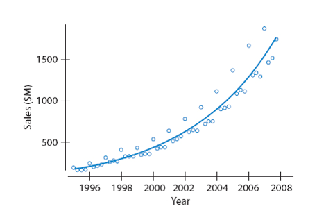
Trend Component
The overall pattern in the plot of the time series is called the trend component.
If a series shows no particular trend over time and has a relatively consistent mean, it is said to be stationary in the mean.
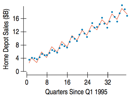
Seasonal Component
The seasonal component of a time series is the part of the variation that fluctuates in a way that is roughly stable over time with respect to timing, direction, and magnitude.
A deseasonalized, or seasonally adjusted series is one from which the seasonal component has been removed.
The time between peaks of a seasonal component is referred to as the period.
Cyclical Component
Regular cycles in the data with periods longer than one year are referred to as cyclical components.
When a cyclical component can be related to a predictable phenomenon, then it can be modeled based on some regular behavior and added to whatever model is being built for the time series.
Irregular Component
In time series modeling, the residuals – the part of the data not fit by the model – are call the irregular component.
Typically the variability of the irregular component is of interest – whether the variability changes over time or whether there are any outliers or spikes that may deserve special attention.
A time series that has a relatively constant variance is said to be stationary in the variance.
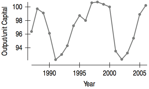
Example 1
Data from the U.S. Bureau of Labor gives Output/hr Labor and Output/unit Capital. Analyze the time series plot below.
Describe the Trend component.
Horizontal
Is there evidence of a Seasonal component?
No strong evidence of a Seasonal component.
Is there evidence of a cyclic component?
Yes, there is evidence of a cyclic component.
Modeling Time Series
Methods for forecasting a time series fall into two general classes: smoothing methods and regression-based modeling methods.
Although the smoothing methods do not explicitly use the time series components, it is a good idea to keep them in mind. The regression models explicitly estimate the components as a basis for building models.
Smoothing Methods
Most time series contain some random fluctuations that vary up and down rapidly that are of no help in forecasting.
To forecast the value of a time series, we want to identify the underlying, consistent behavior of the series.
The goal in smoothing is to "smooth away" the rapid fluctuations and capture the underlying behavior.
Often, recent behavior is a good indicator of behavior in the near future.
Smoothing out fluctuations is generally accomplished by averaging adjacent values in the series.
Simple Moving Average Methods
The Moving Average replaces each value in a time series by an average of the adjacent values.
The number of values used to construct each average is called the length (L) of the moving average.
A moving average of length L, denoted MA(L), simply uses the mean of the previous L actual values as the fitted value at each time.
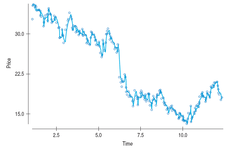
Example 2
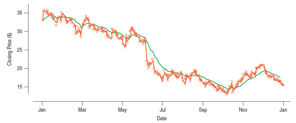
Consider the plot of a time series for the closing price of a stock over the course of a year.
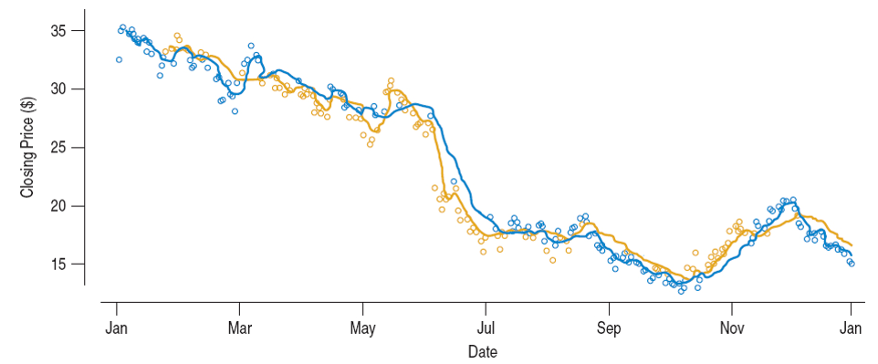
The forecasted values for MA(5) (blue) and MA(15) (brown) are plotted below. Note that the longer moving average is smoother but reacts to rapid changes in the data more slowly.
Simple Moving Average Methods (cont.)
To obtain a forecast for a new time point, analysts use the last average in the series.
This is the simple moving average forecast.
It is the simplest forecast, called the naïve forecast, and it can only forecast one time period into the future.
Moving averages are often used as summaries of how a time series is changing. Outliers tend to affect means and may distort the moving average summary.
Weighted Moving Averages
A weight can be assigned to each value in a weighted averaging scheme according to how far it is before the current value. Each value is multiplied by a weight before summing, and the total is divided by the sum of the weights.
Two types of weighted moving average smoothers are commonly used on time series data: exponential smoothers and autoregressive moving averages.
Exponential Smoothing Methods
Exponential smoothing is a weighted moving average with weights that decline exponentially into the past.
This model is called the single-exponential smoothing model (SES).
All previous values are used in exponential smoothing with distant values getting increasingly smaller weight. This can be seen by expanding the equation above to obtain the equation below.
Example 3
Below we see a plot of the closing price of a stock (data shown in earlier slide) with exponentially smoothed values using $\alpha = 0.75$ (brown) and $\alpha = 0.10$ (green).
Forecast Error
We define the forecast error at any time $t$ as:
To consider the overall success of a model at forecasting for a time series we can use the mean squared error (MSE).
Forecast Error (cont.)
The MSE penalizes large errors because the errors are squared, and it is not in the same units as the data. We address these issues by defining the mean absolute deviation (MAD).
Forecast Error (cont.)
The most common approach to measuring forecast error compares the absolute errors to the magnitude of the estimated quantity. This leads to what is called the mean absolute percentage error (MAPE).
Autoregressive Models
Simple moving averages and exponential smoothing methods are good choices for series with no regular long-term patterns.
If such patterns are present, we may want to choose weights that facilitate modeling that structure.
To find the weights, we can use the methods of multiple regression.
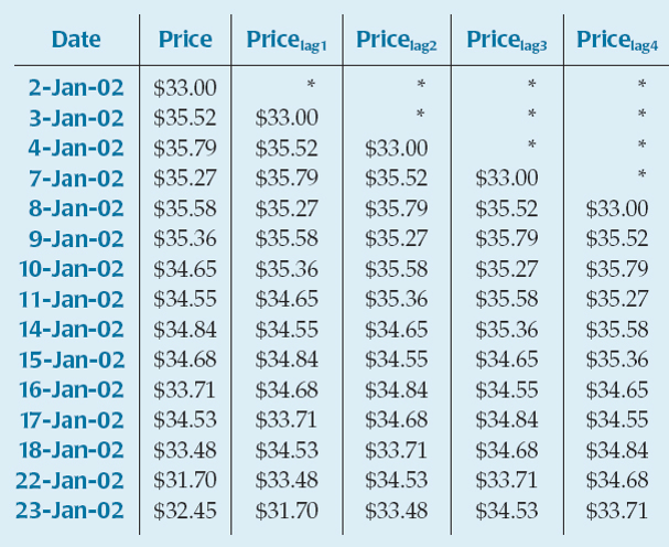
We do so by shifting the data by a few time periods, a process know as lagging which leads to the lagged variables.
A regression is fit to the data to predict a time series from its lagged variables.
Autoregressive Models (cont.)
If we fit a regression to predict a time series from its lag1 and lag2 versions,
Autoregressive Models (cont.)
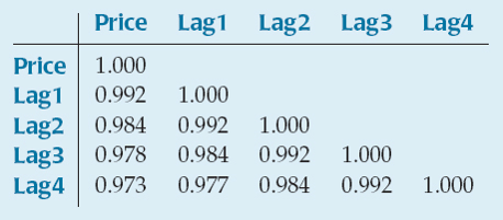
The correlation between a series and a (lagged) version of the same series that is offset by a fixed number of time periods is called autocorrelation. The table shows some autocorrelations for the previous example.
Autoregressive Models (cont.)
A regression model that is based on an average of prior values in the series weighted according to a regression on lagged version of the series is called an autoregressive model.
A pth-order autoregressive model has the form
Example 4
For the closing price of a stock data and its four lag variables in a previous slide, we find the coefficients for a fourth-order autoregressive model.
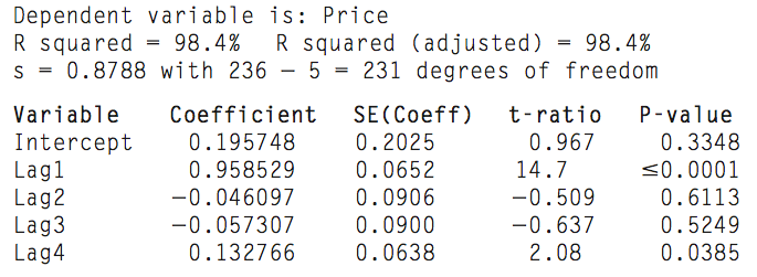
Because a fourth-order model is created, the model can be used to predict four time periods into the future.
Example 4 (cont.)
From the table in the previous slide, we obtain the following fourth-order autoregressive model.
Random Walks
The naïve forecast model is sometimes called a random walk because each new value can be thought of as a random step away from the previous value.
Time series modeled by a random walk can have rapid and sudden changes in direction, but they also may have long periods of runs up or down that can be mistaken for cycles.
where $\varepsilon_i$ are independent random values with some distribution.
Multiple Regression-based Models
The models studied so far do not attempt to model these components directly. Modeling the components directly can have two distinct advantages.
The ability to forecast beyond the immediate next time period.
The ability to understand the components themselves and reach a deeper understanding of the time series.
Modeling the Trend Component
When a time series has a linear trend, it is natural to model it with a linear regression of $y_t$ on Time.
The residuals would then be a detrended version of the time series.
Attractive feature of a regression-based model:
The coefficient of Time can be interpreted directly as the change in y per time unit.
When the time series doesn’t have a linear trend, we can often improve the linearity of the relationship with a re-expression of the data.
The re-expression most often used with time series is the logarithm.
Additive and Multiplicative Models
Adding dummy variables to the regression of a time series on Time turns what was a simple one-predictor regression into a multiple regression.
If we model the original values, we have added the seasonal component, S, (in the form of dummy variables) to the trend component, T, (in the form of an intercept coefficient and a regression with the Time variable as a predictor).
This is an additive model because the components are added in the model.
Additive and Multiplicative Models (cont.)
After re-expressing a time series using the logarithm, we can still find a multiple regression. Because we are modeling the logarithm of the response variable, the model components are multiplied and we have a multiplicative model
Although the terms in a multiplicative model are multiplied, we always fit the multiplicative model by taking logarithms, changing the form to an additive model that can be fit by multiple regression.
Using Cyclical and Irregular Components
Time series models that are additive over their trend component, seasonal component, cyclical component, and irregular components may be written
Time series models that are multiplicative over their trend component, seasonal component, cyclical component, and irregular components may be written
Forecasting with Regression-based Models
Regression models are easy to use for forecasting, and they can be used to forecast beyond the next time period. The uncertainty of the forecast grows the further we extrapolate.
The seasonal component is the most reliable part of the regression model. The patterns seen in this component can probably be expected to continue into the future.
The trend component is less reliable since the growth of real-world phenomena cannot be maintained indefinitely.
The reliability of the cyclical component for forecasting must be based on one’s understanding of the underlying phenomena.
Choosing a Time Series Forecasting Method
Simple moving averages demand the least data and can be applied to almost any time series. However:
They forecast well only for the next time period.
They are sensitive to spikes or outliers in the series.
They don’t do well on series that have a strong trend.
Choosing a Time Series Forecasting Method (cont.)
Exponential smoothing methods have the advantage of controlling the relative importance of recent values relative to older ones. However:
They forecast well only for the next time period.
They are sensitive to spikes or outliers in the series.
They don’t do well on series that have a strong trend.
Choosing a Time Series Forecasting Method (cont.)
Autoregressive moving average models use automatically determined weights to allow them to follow time series that have regular fluctuations. However:
They forecast for a limited span, depending on the shortest lag in the model.
They are sensitive to spikes or outliers in the series.
Choosing a Time Series Forecasting Method (cont.)
Regression-based models can incorporate exogenous variables to help model business cycles and other phenomena. They can also be used to forecast into the future. However:
You must decide whether to fit an additive model or to re-express the series by logarithms and fit the resulting multiplicative model.
These models are sensitive to outliers and failures of linearity. Seasonal effects must be consistent in magnitude during the time covered by the data.
Forecasts depend on the continuation of the trend and seasonal patterns.