Lecture 13
Outline
Observational Studies and Experiments
The Four Principals of Experimental Design
Issues in Experimental Designs
The One-Way Analysis of Variance
Assumptions and Conditions for ANOVA
Observational Studies and Experiments
A statistical study is observational when it is conducted using pre-existing data—collected without any particular design.
An observational study is retrospective if it studies an outcome in the present by examining historical records.
An observational study is prospective if it seeks to identify subjects in advance and collects data as events unfold.
Randomized, Comparative Experiments
An experiment is a study in which the experimenter manipulates attributes of what is being studied and observes the consequences.
The attributes, called factors, are manipulated by being set to particular levels and then allocated or assigned to individuals.
An experimenter identifies at least one factor to manipulate and at least one response variable to measure.
The combination of factor levels assigned to a subject is called that subject's treatment.
Example 1
A soft-drink company wants to compare the formulas it has for their cola product. It created its cola with different types of sweeteners (sugar, corn syrup, and an artificial sweetener). All other ingredients and amounts were the same. Ten trained testers rated the colas on a scale of 1 to 10. The colas were presented to each taste tester in a random order.
Identify the experimental units, the treatments, the response, and the random assignment.
Experimental units: Colas
Treatments: Sweeteners
Response: Tester Rating
Random assignment: Colas were presented in a random order.
The Four Principals of Experimental Design
Control
We control sources of variation other than the factors, we are testing, by making conditions as similar as possible for all treatment groups.
An experimenter tries to make any other variables that are not manipulated as alike as possible.
Controlling extraneous sources of variation reduces the variability of the responses, making it easier to discern differences among the treatment groups.
Testing agains some baseline measurement is called a control treatment, and the group that receives it is called the control group.
Randomize
In any true experiment, subjects are assigned treatments at random.
Randomization allows us to equalize the effects of unknown or uncontrollable sources of variation.
Although randomization can't eliminate the effects of these sources, it spreads them out across the treatment levels so that we can see past them.
Replicate
To estimate the variability of our measurements, we must make more than one observation at each level of each factor, making repeated observations.
Some experiments combine two or more factors in ways that may permit a single observation for each treatment, that is, each combination of factor levels.
When such an experiment is repeated in its entirety, or replicated. Repeated observations at each treatment are called replicates.
Replication can be done for the entire experiment for a different group of subjects, under different circumstances, or at a different time.
Replication in a variety of circumstances increase our confidence that results apply to other situations and populations.
Blocking
Group or block subjects together according to some factor that you cannot control and feel may affect the response. Such factors are called blocking factors, and their levels are called blocks.
Example blocking factors: sex, ethnicity, marital status, etc.
In effect, blocking an experiment into $n$ blocks is equivalent to running $n$ separate experiments.
Blocking in an experiment is like stratifying in a survey design.
Blocking reduces variation by comparing subjects within these more homogenous groups.
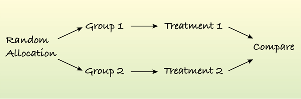
Completely Randomized Design
When each of the possible treatments is assigned to at least one subject at random, the design is called a completely randomized design.
This design is the simplest and easiest to analyze of all experimental designs.
Randomized Block Designs
When one of the factors is a blocking factor, complete randomization isn't possible.
We can't randomly assign factors based on people's behavior, age, sex, and other attributes.
We may want to block by these factors in order to reduce variability and to understand their effect on the response.
When we have a blocking factor, we randomize the subject to the treatments within each block. This is called a randomized block design.
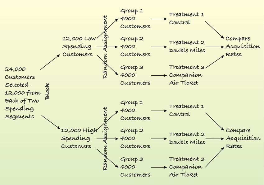
Example 2
In the following experiment, a marketer wanted to know the effect of two types of offers in each of two segments: a high spending group and a low spending group. The marketer selected 12,000 customers from each group at random and then randomly assigned the three treatments to the 12,000 customers in each group so that 4000 customers in each segment received each of the three treatments. A display makes the process clearer.
Example 2 (cont.)
Factorial Designs
An experiment with more than one manipulated factor is called a factorial design.
A full factorial design contains treatments that represent all possible combinations of all levels of all factors.
When the combination of two factors has a different effect than you would expect by adding the effects of the two factors together, that phenomenon is called an interaction.
If the experiment does not contain both factors, it is impossible to see interactions.
Issues in Experimental Designs
Blinding
Blinding is the deliberate withholding of the treatment details from individuals who might affect the outcome.
Two sources of unwanted bias:
Those who might influence the results (the subjects, treatment administrators, technicians, etc.)
Those who evaluate the results (judges, experimenters, etc.)
Single-Blind Experiment: one or the other groups is blinded. Double-Blind Experiment: both groups are blinded.
Placebos
Often simply applying any treatment can induce an improvement. Some of the improvement seen with a treatment—even an effective treatment—can be due simply to the act of treating. To separate these two effects, we can sometimes use a control treatment that mimics the treatment itself.
A "fake" treatment that looks just like the treatments being tested is called a placebo.
Placebos are the best way to blind subjects so they don't know whether they have received the treatment or not.
Confounding Variables
When the levels of one factor are associated with the levels of another factor, we say that two factors are confounded.
Example: A bank offers credit cards with two possible treatments:
low rate and no fee
high rate and 50 dollar fee
There is no way to separate the effect of the rate factor from that of the fee factor. These two factors are confounded in this design.
Confounding and Lurking Variables
A lurking variable "drives" two other variables in such a way that a causal relationship is suggested between the two.
Confounding occurs when levels incorporate more than one factor. The confounder does not necessarily "drive" the companion factor(s) in the level.
Example 3
A wine distributor presents the same wine in two different glasses to a group of connoisseurs. Each person was presented an envelope with two different prices for the wine corresponding to the glass and were asked to rate the taste of the two “different” wines. Is this experiment single-blind, double-blind, or not blinded at all. Explain.
This experiment is double-blinded since the administrators of the taste test did not know which wine the taster thought was more expensive and the tasters were not aware that the two wines were the same, only that the two wines were the same type.
The One-Way Analysis of Variance
Consider an experiment with a single factor of $k$ levels.
Question of Primary Interest:
Is there evidence for differences in effectiveness for the treatments?
Let $\mu_i$ be the mean response for treatment group $i$. Then, to answer the question, we must test the hypothesis:
The One-Way Analysis of Variance (cont.)
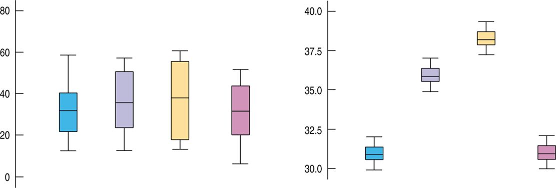
What criterion might we use to test the hypothesis?
The test statistic compares the variance of the means to what we'd expect that variance to be based on the variance of the individual responses.
The differences among the means are the same for the two sets of boxplots, but it's easier to see that they are different when the underlying variability is smaller.
The One-Way Analysis of Variance (cont.)
The F-statistic compares two measures of variation, called mean squares.
The numerator measures the variation between the groups (treatments) and is called the Mean Square due to Treatments (MST).
The denominator measures the variation within the groups, and is called the Mean Square due to Error (MSE).
F_{k-1,N-k} = \frac{MST}{MSE}$
Every F-distribution has two degrees of freedom, corresponding to the degrees of freedom for the mean square in the numerator and the denominator.
Mean Square due to Treatments (MST)
The Mean Square due to Treatments (between-group variation measure)
where $\bar{y}_i$ is a mean for group $i$, $\bar{\bar{y}}$ is a grad mean (for all data), $n_i$ observations in group $i$.
Mean Square due to Error (MSE)
The Mean Square due to Error (within-group variation measure)
where $s_i$ is a variance for group $i$, $n_i$ observations in group $i$, $N$ is a total number of observations.
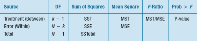
Analysis of Variance
This analysis is called an Analysis of Variance (ANOVA), but the hypothesis is actually about means.
The null hypothesis is that the means are all equal.
The collection of statistics—the sums of squares, mean squares, F-statistic, and P-value—are usually presented in a table, called the ANOVA table, like this one:
Example 4
Tom's Tom-Toms tries to boost catalog sales by offering one of four incentives with each purchase:
Free drum sticks
Free practice pad
Fifty dollars off any purchase
No incentive (control group)
Example 4 (cont.)
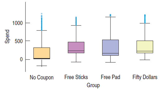
Here is a summary of the spending for the month after the start of the experiment. A total of 4000 offers were sent, 1000 per treatment.
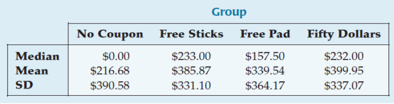
Example 4 (cont.)
Use the summary data to construct an ANOVA table.
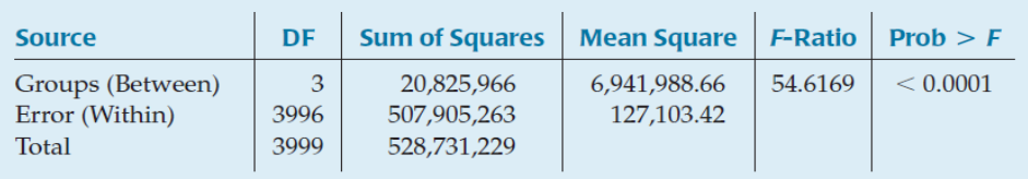
Since $P$ is so small, we reject the null hypothesis and conclude that the treatment means differ.
The incentives appear to alter the spending patterns.
Assumptions and Conditions for ANOVA
Independence Assumption
The groups must be independent of each other.
No test can verify this assumption. You have to think about how the data were collected and check that the Randomization Condition is satisfied.
Equal Variance Assumption
ANOVA assumes that the true variances of the treatment groups are equal. We can check the corresponding Similar Variance Condition in various ways:
Look at side-by-side boxplots of the groups. Look for differences in spreads.
Examine the boxplots for a relationship between the mean values and the spreads. A common pattern is increasing spread with increasing mean.
Look at the group residuals plotted against the predicted values (group means). See if larger predicted values lead to larger-magnitude residuals.
Normal Population Assumption
Like Student's t-tests, the F-test requires that the underlying errors follow a Normal model. As before when we faced this assumption, we’ll check a corresponding Nearly Normal Condition.
Examine the boxplots for skewness patterns.
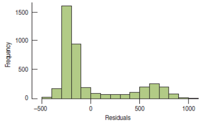
Examine a histogram of all the residuals.
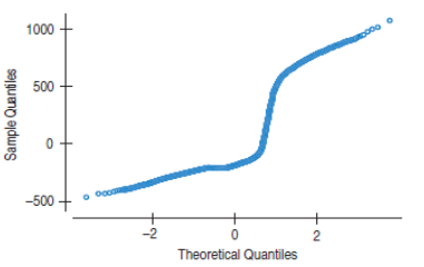
Example a Normal probability plot.
Example 4 (cont.)
For the Tom's Tom-Toms experiment, the residuals are not Normal. In fact, the distribution exhibits bimodality.
Example 4 (cont.)
The bimodality shows up in every treatment!
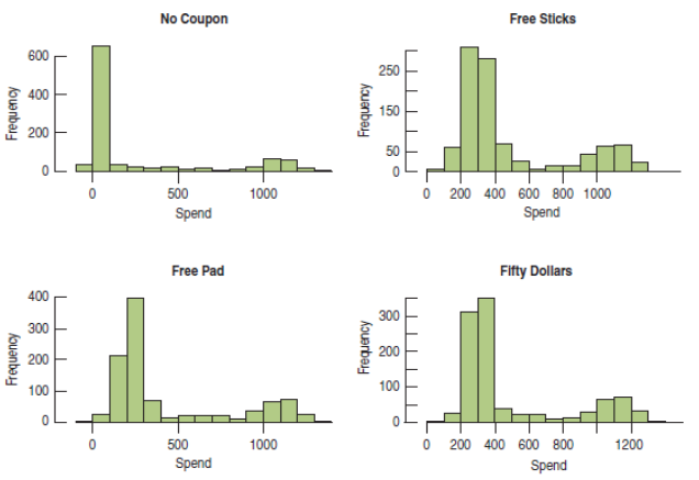
This bimodality came as no surprise to the manager.
"...customers...either order a complete new drum set, or...accessories...or choose not to purchase anything."
Example 4 (cont.)
These data (and the residuals) clearly violate the Nearly Normal Condition. Does that mean that we can't say anything about the null hypothesis?
No. Fortunately, the sample sizes are large, and there are no individual outliers that have undue influence on the means. With sample sizes this large, we can appeal to the Central Limit Theorem and still make inferences about the means.
In particular, we are safe in rejecting the null hypothesis.