Lecture 6

Outline

Confidence Intervals for Proportions
Confidence Intervals for Means

Confidence Interval for Proportions

A Confidence Interval (Example)

In March 2010, a Gallop Poll found that 1012 out of 2976 respondents thought economic conditions were getting better – a sample proportion of

\[\hat{p} = 1012/2976 = 34.0\%\]

We’d like use this sample proportion to say something about what proportion, $p$, of the entire population thinks the economic conditions are getting better.

A Confidence Interval (cont.)

We know that our sampling distribution model is centered at the true proportion

\[SD = \sqrt \frac{pq}{n}, q = 1-p\]

So, following CLT, we can aproximate the sampling distribution with Normal, and use $\hat{p}$ to calculate SE.

\[SE(\hat{p}) = \sqrt \frac{\hat{p}\hat{q}}{n} = \sqrt \frac{(0.34)(1-0.34)\hat{q}}{2976} = 0.009\]

A Confidence Interval (cont.)

Because the distribution is Normal, we expect that about 95% of all samples of 2976 U.S. adults would have had sample proportions within two SEs of $p$, 0.0018.

"It is probably true that 34.0% of all U.S. adults thought the economy was improving."
- We can be pretty certain that whatever the true proportion is, it’s probably not exactly 34.0%.
"We don't know the exact proportion of U.S. adults who thought the economy was improving but the interval from 32.2% to 35.8% probably contains the true proportion."
- This is close to correct, but what is meant by probably?

A Confidence Interval (cont.)

An appropriate interpretation of our confidence interval would be,

"We are 95% confident that between 32.2% to 35.8% of U.S. adults thought the economy was improving."

The confidence interval calculated and interpreted here is an example of a one-proportion z-interval.

What Does "95% Confidence" Really Mean?

Our uncertainty is about whether the particular sample we have at hand is one of the successful ones or one of the 5% that fail to produce an interval that captures the true value.

conf-int

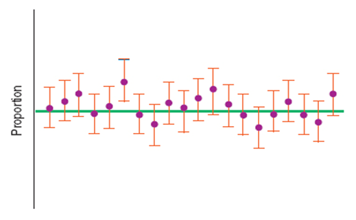
We know the sample proportion varies from sample to sample. If other pollsters would have collected samples, their confidence intervals would have been centered at the proportions they observed.

Margin of Error: Certainty vs. Precision

Our confidence interval can be expressed as below.

\[\hat{p} \pm 2SE(\hat{p})\]

The extent of that interval on either side of is called the margin of error (ME). The general confidence interval can now be expressed in terms of the ME.

\[estimate \pm ME\]

The more confident we want to be, the larger the margin of error must be.
Every confidence interval is a balance between certainty and precision.

Critical Values

For any confidence level the number of SEs we must stretch out on either side of $\hat{p}$ is called the critical value.

Because a critical value is based on the Normal model, we denote it $z^*$.

|CI|$z^*$| |–|––-| |90%|1.645| |95%|1.960| |99%|2.576|

In the spring of 2009 workers at Sony France protesting layoffs, took the boss hostage, "bossnapping". What did other French adults think of this practice? Where they sympathetic? Understanding? Approving?

A polls taken in April 2009 found:

30% “approving”,
63% were “understanding” or “sympathetic” of the action,
Only 7% condemned the practice of "bossnapping"

The poll was based on a random representative sample of 1010 adults.

Example 1 (cont.)

Conditions:

Randomization Condition: The sample was selected randomly.
10% Condition: The sample is certainly less than 10% of the population.
Success/Failure Condition:

\[n\hat{p} = (1010)*(0.63) = 636 \geq 10\]

\[n\hat{q} = (1010)*(0.37) = 374 \geq 10\]

The conditions are satisfied so a one-proportion z-interval using the Normal model is appropriate.

Example 1 (cont.)

What can we conclude about the proportion of all French adults who sympathize?

\[n = 1010, \hat{p} = 0.63\]

\[SE(\hat{p}) \sqrt \frac{(0.63)(0.37)}{1010} = 0.015\]

For a 95% CI, $z^* = 1.96$, so

\[ME = z^* SE(\hat{p}) = 1.96(0.015) = 0.029\]

\[0.63 \pm 0.029\]

Based on the survey we can be 95% confident that between 60.1% and 65.9% of all French adults were sympathetic.

Choosing the Sample Size

To get a narrower confidence interval without giving up confidence, we must choose a larger sample.

\[ME = z^* \sqrt \frac{\hat{p}\hat{q}}{n}\]

Thus,

\[n = (z^*)^2 \frac{\hat{p}\hat{q}}{ME^2}\]

Example 2

Suppose a company wants to offer a new service and wants to estimate, to within 3%, the proportion of customers who are likely to purchase this new service with 95% confidence. How large a sample do they need?

We proceed by guessing the worst case scenario for $\hat{p}$. We guess $\hat{p}$ is 0.50 because this makes the SD (and therefore n) the largest.

\[n = (1.96)^2 \frac{(0.5)(0.5)}{0.03^2} = 1067.1\]

We can conclude that the company will need at least 1068 respondents to keep the margin of error as small as 3% with confidence level 95%.

Confidence Intervals for Means

The Sampling Distribution for the Mean

Confidence intervals for proportions to be

\[\hat{p} \pm ME\]

where the $ME$ was equal to a critical value, $z^*$, times $SE(\hat{p})$.

Confidence intervals means will be

\[\bar{y} \pm ME\]

where the $ME$ was equal to a critical value, $z^*$, times $SE(\bar{y})$.

The Sampling Distribution for the Mean (cont.)

Because the true value of the population standard deviation $\sigma$ is unknown.

Instead of $\sigma$, we will use $s$, the sample standard deviation from the data. So, $SE(\bar{y}) = \frac{s}{\sqrt n}$

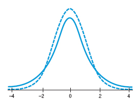
Gosset's t

William S. Gosset discovered above when he used the standard error $\frac{s}{\sqrt n}$ the shape of the curve was no longer Normal.

New model was called the Student's t, and it is always bell-shaped, but the details change with the sample sizes.

The Student's t-models form a family of related distributions depending on a parameter known as degrees of freedom.

t-dist

Example 3

Data from a survey of 25 randomly selected customers found a mean age of 31.84 years and the standard deviation was 9.84 years.

What is the standard error of the mean?

How would the standard error change if the sample size had been 100 instead of 25? (Assume that $s$ = 9.84 years.)

Practical sampling distribution model for means

When certain conditions are met, the standardized sample mean,

\[t = \frac{\bar{y} - \mu}{SE(\bar{y})}\]

follows a Student's t-model with $n-1$ degrees of freedom. We find the standard error from:

\[SE(\bar{y}) = \frac{s}{\sqrt n}\]

One-sample t-interval

When the assumptions and conditions are met, the confidence interval for the population mean, $\mu$ is:

\bar{y} \pm t^*_{n-1} \times SE(\bar{y})$

The critical value $t^*_{n-1}$ depends on the particular confidence level, $C$, that you specify and on the number of degrees of freedom, $n-1$, which we get from the sample size.

Finding t-values

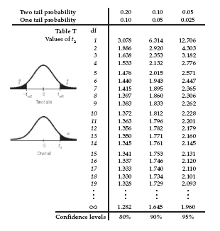t-dist For example, suppose we’ve performed a one-sample t-test with 19 df and a critical value of 1.639, and we want the upper tail P-value.

From the table, we see that 1.639 falls between 1.328 and 1.729. All we can say is that the P-value lies between P-values of these two critical values, so 0.05 < P < 0.10.

Example 4

Data from a survey of 25 randomly selected customers found a mean age of 31.84 years and the standard deviation was 9.84 years.

Construct a 95% confidence interval for the mean. Interpret the interval.

Example 4 (cont.)

Construct a 95% confidence interval for the mean.

\[\bar{y} \pm t^*_{n-1} \times SE(\bar{y}) = 31.84 \pm (2.064)(1.968) =\]

\[31.84 \pm 4.062 = (27.78, 35.90)\]

Interpret the interval.

We're 95% confident the true mean age of all customers is between 27.78 and 35.90 years.

Assumptions and Conditions

Independence Assumption: There is no way to check independence of the data, but we should think about whether the assumption is reasonable.
Randomization Condition: The data arise from a random sample or suitably randomized experiment.
10% Condition: The sample size should be no more than 10% of the population. For means our samples generally are, so this condition will only be a problem if our population is small.
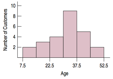
Nearly Normal Condition: The data come from a distribution that is unimodal and symmetric. This can be checked by making a histogram.

Normal Population Assumption

For very small samples (n < 15), the data should follow a Normal model very closely. If there are outliers or strong skewness, t-methods shouldn’t be used.
For moderate sample sizes (n between 15 and 40), t-methods will work well as long as the data are unimodal and reasonably symmetric.
For sample sizes larger than 40 or 50, t-methods are safe to use unless the data are extremely skewed. If outliers are present, analyses can be performed twice, with the outliers and without.

Example 5

In 25 randomly selected customers survey found a mean age of 31.84 years and the standard deviation was 9.84 years. A 95% confidence interval for the mean is (27.78, 25.90).

Independence: Data were gathered from a random sample and should be independent.
10% Condition: These customers are fewer than 10% of the customer population.
Nearly Normal: The histogram is unimodal and approximately symmetric.

Degrees of Freedom: Why n – 1?

If we know the true population mean, $\mu$, we can find the standard deviation using $n$ instead of $n – 1$.

\[s = \sqrt \frac{(y - \mu)^2}{n}\]

For any sample, $\bar{y}$ will be as close to the data values as possible, and the population mean μ will be farther away.

If we use $\sum (y - \bar{y})^2$ instead of $\sum (y - \mu)^2$ in the equation to calculate s, our standard deviation will be too small.

We compensate for this by dividing by $n – 1$ instead of by $n$.